2D elements

This entry takes a closer look at different 2D element types, and the options for modelling 2D element results in GSA.

2D element types

In GSA, 2D elements are relatively simple elements defined by:

1. Shape
2. Order
3. Type

1. Shape

Quad or triangle.

Tip: Avoid triangular elements where quad elements can be used, as triangular elements are generally less efficient and accurate.

2. Order

Linear (corner nodes only) or parabolic (corner and mid-size nodes).

3. Type

The two most used 2D element types in GSA are the plane stress element and the shell element.

Plane stress element

• No variation and no stress through the thickness.
• The state of stress at any point represented by the simplified stress tensor:

$$\begin{bmatrix} \sigma_{xx} & \sigma_{xy} & 0\\ \sigma_{yx} & \sigma_{yy} & 0\\ 0 & 0 & 0 \end{bmatrix}$$

Shell elements

• Assumes no through thickness, direct stress.
• Includes through thickness, shear stress.

The stress tensor reduces to:

$$\begin{bmatrix} \sigma_{xx} & \sigma_{xy} & \sigma_{xz} \\ \sigma_{yx} & \sigma_{yy} & \sigma_{yz} \\ \sigma_{zx} & \sigma_{yz} & 0 \end{bmatrix}$$

The stress tensor varies through the thickness of the element. For a linear model, the stress at the mid-plane can be thought of as the in-plane stress. The difference between the top and bottom stresses is the bending stress.

For a shell element, it is easier to convert these to forces and moments.

2D element mesh

The mesh must be designed so that elements are sufficient to model the actual stiffness of the structure.

The size and shape of the finite elements is determined by:

• The type of element being used
• The shape of the boundary elements and elements that are nearby
• The loading

To ensure that elements are all facing the same way up and properly connected:

1. Select the Section display tool .
2. Check Fill.
3. Then choose the Labels and display methods tool .
4. Select Edge check.
5. In the dialogue box select the Elements/members tab and tick Element edges.

2D element axes

These can be defined either by reference to an axis set (global or user defined axes), using the 2D element property axis, or topologically (local axes).

2D element axes are defined by projecting the 2D element property axis on to the element. If set to Local, set the first edge defining the element x, and the first and last edges defining the element xy plane.

Defining 2D element local axes by reference to an axis set results in more consistent local axes in the mesh. When the 2D element property axis is set to other than local, then the specified axis system is projected on to the element.

Note: Look out for: Local axis definition. Adjacent elements may have completely different axis directions making it difficult to interpret results.

Tip: If you aren’t sure about the orientation of the local axes, tick Element axes in the Labels and display methods dialogue box. The axes are coloured Red / Green / Blue for x / y / z.

2D element results

Key tools and icons

Icon	Function
	Label and display methods
	Labels
	Contours
	Contour settings, (opens contour plot dialogue box)
	Wood-Armer moments
	Axes

Forces and moments

Note: Forces and moments are given per unit length in the relevant direction. These are essentially the appropriate stresses multiplied by the element thickness. For a 0.5 × 0.5m square element, therefore, you need to multiply the $kN/m$ value by 0.5 to get the total $kN$ force in the element.

In-plane forces

The in-plane forces are:

$$N_{x}\; = \int \sigma_{xx}\; dt$$

$$N_{y}\; = \int \sigma_{yy}\; dt$$

$$N_{xy}\; = \int \sigma_{xy}\; dt$$

These correspond to a 2D tensor based on the in-plane stresses aggregated over the thickness of the element.

Moments

The moments are:

$$M_{x}\; = \int \sigma_{xx}\; dz$$

$$M_{y}\; = \int \sigma_{yy}\; zdz$$

$$M_{xy}\; = \int \sigma_{xy}\; zdz$$

These correspond to a 2D tensor based on the bending stresses, aggregated over the thickness of the element.

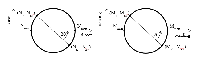
As in-plane forces and moments are tensor quantities we can define principal forces and moment, similar to principal stresses and maximum shear force and twisting moment.

Out-of-plane forces

The remaining terms in the stress tensor contribute to the through thickness forces:

$$\\{Q}_{x}\; = \int \sigma_{xz}\; dt$$

$$\\{Q}_{y}\; = \int \sigma_{yz}\; dt$$

Projected and derived demands

These are the principal demands in whichever direction they occur and can be projected onto an axis of interest.

When you bend a 2D element you get moments about the two in-plane axes ($M_{x}$ and $M_{y}$) and a twisting moment ($M_{xy}$). These form the basis of projected moments.

Note: Projected refers to the way the output axis set is projected on to the surface of the element.

Maximum and minimum moments are the principal moments, (i.e., projected moments rotated so that the twisting moment is 0).

These are derived; calculated from the basic (projected) moment results and are independent of the axis set.

The same principles apply to the in-plane forces ($N_{x}$, $N_{y}$ & $N_{xy}$ and $N_{max}$ & $N_{min}$).

Note: The projected moments $M_{x}$ and $M_{y}$ are based on the stress in the x and y direction respectively (Timoshenko convention) and are not about the x and y axes.

Projected demands

Projected moments are given relative to the specified axes.

Example: $M_{x}$ gives moments in the direction of (not about) the x axis. Whether this is the local axis for each element, or the global axis for the whole model is very important. Always check which you are using by clicking the Axes button in the Contour plot dialogue box. This is accessed via the Contour settings icon to the right of the graphic interface.

The local x axis is defined in the direction of the first edge you draw in the 2D element.

Max and min forces / moments

Both are signed; the latter refers to principal compression. Look at both results to understand the principal compression/tension regime in each element.

To account for in-plane twisting, use the $M_{x}+M_{xy}$ and $M_{y}+M_{xy}$ results.

Wood-Armer moments

Wood-Armer moments increase the moment by the magnitude of the twisting moment, when calculating resistance by slabs and walls:

$$M_{x,wa} = M_x +sgn M_x|M_{xy}|$$

$$M_{y,wa} = M_y +sgn M_y|M_{xy}|$$

Recommendation for designing reinforcement

For torsional moments, use Wood-Armer moments or preferably, GSA slab design, which also considers in-plane forces.

Reinforcement can be in any two general directions, not necessarily orthogonal.

Note: It is appropriate to band reinforcement in a similar manner to that allowed by design codes, but this must be done by hand.

Do not ignore reinforcement peaks within the perimeter of columns:

Punching shear

$\\{Q}_{max}$ can be defined as:

$$\\{Q}_{max}\; = \sqrt{Q_x^2 + Q_y^2}$$

This will indicate the maximum force / unit length (GSA doesn’t define an equivalent stress) at all locations. There are likely to be large inaccuracies, especially adjacent to point supports.

Stress and force results

2D elements in GSA have both stress results and force results.

Stress results

Important:

• Check the results first without averaging stresses and forces at nodes, to ensure the error is small.
• If using envelopes, check the envelope method used, located towards the bottom of the Contours dialogue box.

The fundamental result for 2D element is the stress state. This is represented by a tensor which can be thought of as a matrix, where each term corresponds to a force per unit area:

$$\begin{bmatrix} \sigma_{xx} & \sigma_{xy} & \sigma_{xz} \\ \sigma_{yx} & \sigma_{yy} & \sigma_{yz} \\ \sigma_{zx} & \sigma_{yz} & \sigma_{zz} \end{bmatrix}$$

Where the shear terms may be denoted by $\tau$ instead of $\sigma$

Mohr's circle

We can use Mohr’s circle to understand what is happening in the element, and to the principal stresses.

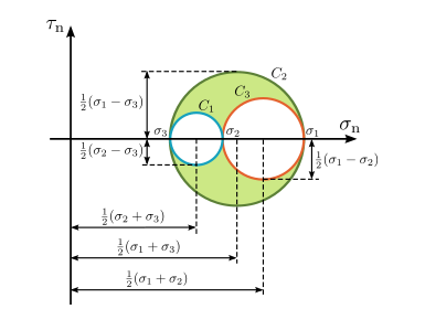
The three circles correspond to the three pairs of directions x-y, y-z and z-x.

Taking the x-y directions, the centre of the circle is:

$$\sigma_c = \frac{\sigma_{xx} + \sigma_{yy}}{2}$$

And the radius:

$$\sigma_{r} = \sqrt{(\sigma_{xx} - \sigma_{c})^2} + \sigma_{xy}^2$$

Giving principle stresses:

$$\sigma_1 = \sigma_{c} + \sigma_{r}$$

$$\sigma_2 = \sigma_{c} - \sigma_{r}$$

The same applies to the other two direction pairs leading to $\sigma1$, $\sigma2$­ and $\sigma3$: maximum, intermediate and minimum principal stresses.

The maximum shear stress is simply the largest value of $\sigma{r}$. Plotting the principal stresses give a good indication of the flow of the stresses in the model, but there are still multiple values to consider.

Taking an element with an isotropic material under uniaxial stress we can measure how close to yielding we are by comparing the stress $\sigma_{xx}$ in the element with the yield stress in the material. To compare the general stress state to yield we normally use the von Mises stress.

This is defined as:

$$\sigma = \sqrt{\frac{1}{2}[(\sigma_{xx} - \sigma_{yy})^2 + (\sigma_{yy} - \sigma_{zz})^2 + (\sigma_{zz} + \sigma_{xx})^2]+3(\sigma_{xy}^2 + \sigma_{yz}^2 + \sigma_{zx}^2)}$$

And in the uniaxial stress state reduces to:

$$\sigma_{v} = \sigma_{xx}$$

Note: GSA RC design will check if your walls can be reinforced. See Projected demands to do independent checks by hand. To check shear stresses use the projected stresses. Normally, GSA sets the element axes with y vertical and x horizontal and z out-of-plane. So, the shear stresses that you are interested in are projected xy. A quick hand calculation to check approximate stresses at, e.g., ground level, should confirm that you are looking at the right thing.