
# Mapped loads
# Mapping beam loads on 1D elements
First, confirm that the layer is set to the Analysis layer (shown on the top right of the graphic window).
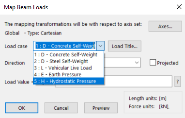
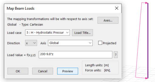
To map loads onto 1D elements, select the desired 1D element(s) to map loads to, and then go to Sculpt > Create element loading > Map beam loads on 1D elements… for the load application window.
- Assign the mapped load to its corresponding load case with the dropdown menu beside Load case.
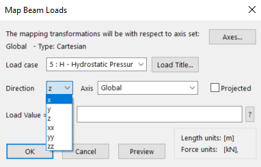
- Assign the desired direction of the mapped load. This is the axis that the load will be applied along.
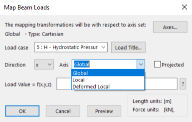
- Assign the desired axis of the mapped load. If custom axes have been defined, they can be selected here.
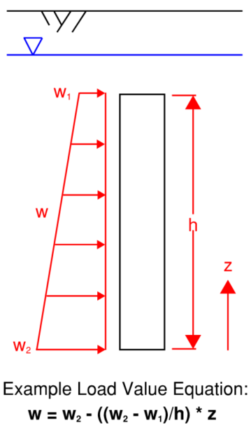
Determine the loading equation to input as the mapped load’s load value. The load value has two components; its application direction and its variable axis.
As an example, if we are applying a horizontal hydrostatic pressure to a vertical 1D element, we can determine the load value at any node along the element with two components. The load would be applied along the horizontal axis (x or y if global axis) – we have already assigned this in steps 4 and 5.
We also need the magnitude of that load, which would be determined based on the vertical coordinate (z if global axis) of that node in this case. Thus, we assign a linear function for the load with ‘z’ as a variable.
In this example, we will use the load value at 0 height and the slope of the linear function. As shown below, w2, w1, and h are calculated values. ‘z’ is a variable that is referring to the z-axis of the coordinate axis specified. As z changes, the load value changes as well (in this case, w decreases as z increases).
Be mindful of positive and negative load directions!
- After the mapped loading has been added, we can preview the load diagram.
If it looks accurate, we can click OK to apply the mapped loading.
After creating the loading, we need to confirm our load values are correct. We do this by turning on load diagrams and changing to the mapped load case.
- We then click Select for annotation (a) on the sidebar or press ‘a’ on our keyboard to annotate results. Next, we select the element(s) to display its load values for the selected load case – if they appear as expected, we have finished applying our mapped loads.
# Mapping face loads on 2D elements
First, confirm that the layer is set to the Analysis layer (shown on the top right of the graphic window).
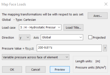
To map loads onto 2D elements, select the desired 2D element(s) to map loads to, and then go to Sculpt > Create element loading > Map face loads on 2D elements… for the load application window.
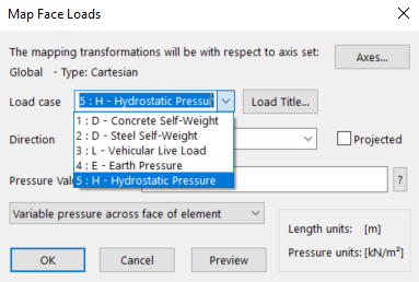
- Assign the mapped load to its corresponding load case with the dropdown menu beside Load case.
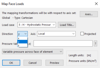
- Assign the desired direction of the mapped load. This is the axis that the load will be applied along.
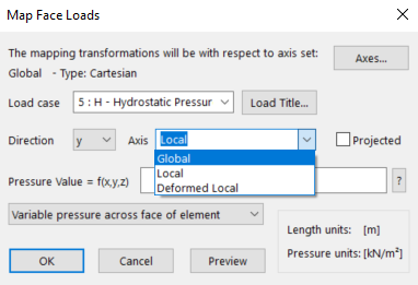
- Assign the desired axis of the mapped load. If custom axes have been defined, they can be selected here.
Determine the loading equation to input as the mapped load’s load value. The load value has two components; its application direction and its variable axis.
As an example, if we are applying a horizontal hydrostatic pressure to a vertical 2D element, we can determine the load value at any node along the element with two components. The load would be applied along the horizontal axis (x or y if global axis) – we have already assigned this in steps 4 and 5.
We also need the magnitude of that load, which would be determined based on the vertical coordinate (z if global axis) of that node in this case. Thus, we assign a linear function for the load with ‘z’ as a variable.
In this example, we will use the load value at 0 height and the slope of the linear function. As shown below, w2, w1, and h are calculated values. ‘z’ is a variable that is referring to the z-axis of the coordinate axis specified. As z changes, the load value changes as well (in this case, w decreases as z increases).
Note: Be mindful of positive and negative load directions!
- After the mapped loading has been added, we can preview the load diagram.
If it looks accurate, we can click OK to apply the mapped loading.
After creating the loading, we need to confirm our load values are correct. We do this by turning on load diagrams and changing to the mapped load case.
- We then click Select for annotation (a) on the sidebar or press ‘a’ on our keyboard to annotate results. Next, we select the element(s) to display its load values for the selected load case – if they appear as expected, we have finished applying our mapped loads.
← LS-DYNA