
# Grid Loads
Grid loading is loading applied in space by means of a grid plane. There are three basic types of grid loading: point loads, line loads and area loads. The area loads can be subdivided into loads on the whole grid plane and those on a defined area bounded by a polyline defining a closed polygon. The panels to which the loads are applied can be one-way spanning or two-way spanning or multi-way spanning.
# Grid Cells
A loading grid is used to integrate area loads and for distribution of grid point loads on to beam elements around the panel. The grid used needs to be fine enough to give an adequate representation of the load, so it needs to be based on the size of the panels that are loaded. The size and shape of the panels can vary significantly, so a robust way of determining the grid size is required.
For a square panel the load can probably be represented adequately by a 4 × 4 grid, but for a long thin panel the same grid would be unsuitable. The grid size is established as follows:
Calculate the area of the panel and set a representative panel dimension to be the square root of this. Then the grid size is this value divided by the grid refinement factor. This defaults to give typically 4 cells along the edge of a square panel. The user can adjust the grid refinement factor to a lower or higher value if required.
For a series of aspect ratios with a refinement factor of 4 the mesh densities are as follows.
| Aspect ratio | Cell density |
|---|---|
| 1 : 1 | 4 × 4 |
| 1 : 2 | 2.83 × 5.65 |
| 1 : 4 | 2 × 8 |
| 1 : 10 | 1.265 × 12.65 |
| 1 : 16 | 1 × 16 |
The calculation of the loading grid size can then be calculated on a
panel by panel basis and the final size selected to give adequate
representation on the smaller panels, with not being skewed unduly by a
few very small panels. To ensure that this is the case the average,
# Grid Point Loads
The way in which the loads are applied depends on the type of structure as represented by the span type.
One way spanning loads are calculated by assuming the load applied to a ‘plank’ spanning from one side of the panel to the other in the span direction. In the case of loading over the whole panel this means that the load per ‘plank’ is the product of the load intensity and the plank length, split evenly between each end. The algorithm replaces the plane by a line with a load intensity applied to each end of the line.
The starting point for the two way distribution of load is to consider a
circle of unit radius centred on the load point. The actual intensity at
the edges is calculated by extrapolating from this point using a
We can satisfy these requirements with a distribution of the form
We require that there is force and moment equilibrium. The form of these functions satisfies the moment equilibrium requirement and we can look for a solution for an arbitrary load. The term
takes account of the aspect ratio of the panel in determining the split
between the long and short directions. If the panel is square we expect
the
We then define values as follows:
then we can calculate the coefficients from
The load intensity at the edge of the panel is then calculated from the distance of the point on the edge from the load point.
If we consider a circle at unit radius from the grid point load we have a load intensity function of the form
This must be mapped on to the surrounding elements. We can use the grid
cell size,
The distribution of point loads can then be determined at a series of
point that are a distance c apart along the elements on the boundary
with a minimum of a start and end point on each boundary element. The
number of segments for the load distribution can then be determined from
the grid cell size and element length,
For the default value of grid load refinement and uniform sized square panels this will give four load patches along each side of the panel. The length of the patches is then
Consider two lines from the load point to the start and finish of the
element segment. These will be at angles
where
If the vectors
The loading function contains terms of the form
which integrates to give
The load
and load moment
This point load must then be adjusted to allow for the distance of the
beam from the load point. This can use a
Knowing
# Grid Area Loads
When a grid area load is applied in a multi-spanning panel the approach is to consider the loading to be represented as a grid of “point loads” distributed over the loaded area. The distributed load is then accounted for by summing all the “point loads”.
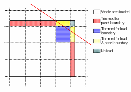
Having established the loading grid size then we can then work through the grid and determine if a cell is loaded or not.
Where a cell is bisected by the load boundary then the load intensity is reduced in proportion to the loaded area and adjustment is made for the position of the load. Where a cell is bisected by the structure boundary the point of application of the load must be moved so that the load is applied to the “structure” and not in “space”. In these cases the centroid of the trimmed loading grid cell is calculated and the (reduced) load on the whole cell applied at the recalculated centroid.
Where a cell is bisected by a panel edge the load is applied to the panel at the centroid of the grid cell.
For the cases where this is too coarse the grid refinement factor can be increased.
Grid area loads can be projected. When this is the case the load
intensity is reduced depending on the projected area of the panel to the
loading axis. If the normal direction of the load is
When the load is not projected then the intensity depend on the panel
area relative to the panel area projected on to the grid plane (normal
When the panels lie in the grid plane this factor is unity.
Note: If a polygon which results in a loaded cell being split into two regions, the whole cell is assumed to be loaded. This results in a (slight) overall increase in the applied load. This restriction is in order to keep the load distribution as fast as possible.
# Grid Line Loads
Grid line loads are treated in a similar manner to grid area loads in that they are broken down into a series of grid point loads along the length of the line. The same grid cell size is used to determine the number of segments along the line and thereafter the procedure is the same as for area loads.