
# Element Stiffness
To generate a stiffness matrix for a curvilinear quadrilateral or triangular element a new approach must be used. Most finite element codes used an approach based on isoparametric or similar elements.
In an isoparametric element the element displacements are interpolated in the same way as the geometry, e.g. a plane stress element. In a superparametric or degenerate isoparametric element the interpolation on the geometry is of a higher order than the interpolation of the displacements, e.g. a plate element. In a subparametric element the interpolation of the geometry is of a lower order than the interpolation of the displacements, e.g. an eight noded straight sided quadrilateral element, where a different geometric interpolation function is used for the geometry from that for the displacements. The term isoparametric is often used as a general term to cover all these element types.
For a plane stress problem, we can establish a material matrix
the strains are
and the stresses are
For an elastic-isotropic material the material matrix is
where
Note that there is an out of plane strain
The strains are defined in terms of the displacements as
The simplest elements to consider are the 4 noded and 8 noded
quadrilateral elements, of which the 4 noded element can be considered a
simplification of the 8 noded element. A typical 8 noded element is
shown below. The element has an arbitrary local coordinate system based
on the location of the nodes and the element property axis
 |  |
|---|
We can set up interpolation functions to interpolate the geometry as follows
where the
These interpolation functions are chosen so that
As the elements are isoparametric we use the same interpolation function for the displacements so the displacement in the element is related to the nodal displacements by
To evaluate the stiffness matrix we need the strain-displacement
transformation matrix. The element displacements are obtained in terms
of derivatives of the element displacements with respect to the local
coordinate system
to establish these derivatives we use the chain rule to set up the following relationship
or in matrix notation
where
This requires that the inverse of the Jacobian exist, which requires that there is a one to one correspondence between natural and local coordinates. This will be the case provided the element is not grossly distorted from a square and that it does not fold back on itself.
We can then evaluate
and thus we can construct the strain-displacement transformation matrix,
where
The elements of
The volume integral is not normally amenable to an explicit integration so normally a numerical integration technique is used. The integral can be written
where
and the integral is performed in the natural coordinate system of the element. This is convenient as the limits of the integration are then ±1. The stiffness can then be calculated
where the matrix
In a similar way the mass matrix and the load vectors are established.
where
# Geometric stiffness matrix of shell element
The geometric stiffness matrix is calculated from:
where
With
and
# 2D Plate Elements
The formulation of 2D plate and shell elements considers both in-plane and transverse (out-of-plane) displacements. Following Mindlin-Reissner plate theory, in addition to the bending strains we consider the effect of transverse shear strain in our complete expression for the element strain
where
We can define separate material matrices
and
respectively.
In this way we can then express the local element stiffness matrix as a summation of the in-plane and out-of-plane stiffness’s
where
While brief, this outlines the basic approach to the Mindlin-Reissner 2D element stiffness formulation. In GSA we label this concisely as the Mindlin formulation.
# MITC Element Formulation
We find that the Mindlin formulation is an effective approach for 2D parabolic elements where the 8-noded element accommodates sufficient terms in the stiffness matrix to sufficiently define the behaviour of the element numerically. However the same formulation defined over a linear element becomes noticeably more problematic where the absence of available terms in our 4-noded stiffness matrix leads to numerical difficulties in expressing the same element behaviour. Specifically we find a difficulty in attempting to represent the transverse shear strain terms. Analytically as before we can express the transverse shear strain as
although numerically, the difference in the order of terms for the shear strain may lead to artificial stiffening of the element where the shear terms are numerically constrained from approaching zero. See reference 1 in the bibliography for further information. This restriction would be particularly noticeable where the thickness of the plate is small.
A widely practiced remedy is to under-integrate the shear term and while effective, its use is at the cost of reduced accuracy and stability for the element. The problem of stability alone is often of greatest concern where the phenomenon of hourglassing can become apparent in elements where the thickness to length ratio is large.
An alternative formulation was put forward by Bathe and Dvorkin and has been found to be especially effective at resolving these difficulties. The formulation is extendable to higher order elements although we find the approach is most effective when resolving the difficulties most apparent in linear elements. The formulation is based upon the theory of Mixed Interpolated Tensoral Components (MITC). For the pure displacement-based Mindlin formulation we use the independent variables
where Bathe now introduces a separate independent variable to represent the transverse shear term
We use
For a linear 2D element we obtain direct values for the shear strain at four points A, B, C, D on the element and so we evaluate the displacement and section rotations at these points through direct interpolation.

We can then construct the interpolations
using direct values for the shear strains obtained at the four points. This replaces our original expression for the shear terms and we continue to construct the local stiffness matrix as normal in a similar approach as before in 2D isoparametric elements. It is lastly worthwhile to note that the interpolation above assumes our element is in the isoparametric coordinate system. Further transformations are necessary to interpolate the shear strains directly through an arbitrary element in local space. Indeed, when this is done the element shows considerably improved predicative capabilities for distorted elements.
# Element shape functions
The element shape functions for 2D elements are
These are for the different element shapes
Tri-3
Quad-4
Tri-6
Quad-8
# 2D Element Shape Checks
A number of element checks are carried out by GSA prior to a GSS analysis. Other analysis programs may have different limits but the same principles apply. For GSS the following warnings, severe warnings and errors are produced.
# Triangle
| Warning | Severe warning | Error |
|---|---|---|
# Quad
| Warning | Severe warning | Error |
|---|---|---|
where
Notes:
The distance out of plane of edge 1 is calculated as
Where
Mid-side node locations not checked but should be approximately halfway along edge.
No check on ratio thickness/shortest side.
# Hourglassing
When Quad 4 elements with the Mindlin formulation are used in bending it is possible to encounter hourglassing problems. This is a problem that arises with under-integrated elements where there are insufficient stiffness terms to fully represent the stiffness of the element. The problem is noticeable in the results by an hourglass pattern in the mesh as shown below.
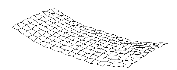
This problem is avoided using the MITC formulation for Quad 4 elements. This formulation uses a separate interpolation method for the transverse shear strains and provides considerably greater stability than the original Mindlin method. The original Mindlin method is kept in GSA for compatibility with previous models although for new models the MITC formulation is recommended.
Alternatively when parabolic accuracy is required Quad 8 elements are recommended. These also formulate elements that are still stiff in all modes of deformation, even when under-integrated.
# 3D Element
The element shape functions for 2D elements are
These are for the different element shapes
Tetra-4
Pyramid-5
Wedge-6
Brick-8
The stiffness matrix for brick elements is obtained using selective
reduced integration to alleviate volumetric locking. The
The dilatational and deviatoric parts of the matrix can be computed using
and
for
# Link Element
Link elements are different to the other element types in that they apply a constraint between a pair of nodes. The primary node is the first node specified in the element topology and this is the node that is retained in the solution. The other node (the constrained node) is related back to the primary node.
The degrees of freedom at the constrained node that are linked will
depend on the type of link. The link allows the constrained node to be
fixed (where the rotations at the constrained node depend on the
rotation of the primary) or pinned (where the rotations at the
constrained node are independent of the rotation of the primary). The
primary node is always has the rotations linked to the rest of the
structure. The links can act in all directions or be restricted to act
in a plane (
The constraint conditions are summarised below:
All directions
Plane (
Loads applied to link elements will be correctly transferred to the primary degree of freedom as a force + moment so no spurious moments result.
The inertia properties of a link element can be calculated from the masses at the nodes attached to the rigid element as follows. The mass is
and the coordinates of the centre of mass are
The inertia about the global origin is then
and relative to the centre of mass
The constraint equations for a link element assume small displacements. When large displacements are applied to a link element the constraint equations no longer apply and the links between constrained and primary get stretched. This effect can be noticeable in a dynamic analysis where the results are scaled to an artificially large value. When these are scaled to realistic value this error should be insignificant.