Footfall analysis

Footfall Analysis with Oasys GSA 10.1

Video timings

The following entry refers to content from the GSA footfall analysis webinar. A list of key sections and timings can be found below:

Timeframe	Description
15:17 - 19:20	General modelling principles
19:22 - 38:00	Live modelling demo
19:22 - 20:11	Drawing members in 3D
20:11 - 20:37	Define material properties
20:37 - 21:37	Define section properties and offsets
21:40 - 22:16	Add loading
22:16 - 22:42	Assign global supports
22:42 -23:19	Create a modal analysis task
23:19 - 24:52	Highest mode frequency
24:52 - 26:22	Check mode shapes
26:22 - 29:38	Create a footfall analysis task
32:29 - 38:00	View footfall analysis results
35:13 - 38:00	Chart output

1. Model setup

Model members

Start modelling by drawing members in 3D.

When drawing the extent of your model, consider the following for:

• Floor plates: Model the entire floor plate to the edge of the building if desired. Alternatively, model the relevant floor bay where vibration results are desired and at least one full bay in each direction around the relevant bay.
• Stairs: Model the entire stair. Model the structure that supports the stair at least one full bay in each direction around the stair to capture the stiffness of the supporting structure itself.
• Columns: Model building columns above and below the relevant floor/stair to capture the stiffness of the columns themselves. Column extents and end fixities are up to the user based on what is most appropriate to capture the realistic stiffness of the columns in the structure.

Define material and section properties

Material properties

To define your material properties, go to the Data tab of the Explorer pane then Materials > Advanced > Material properties.

Note: The effective material modulus for dynamic loading may be different than the typical modulus for static loading. This is typically relevant for concrete floor or composite floor slabs. Reference the relevant design guide for how to calculate the effective concrete modulus for dynamic loading.

Section properties and offsets

Section properties and its offsets can be viewed and edited from Data > Properties > Section library.

_{Image shows section components and offsets dialogs}

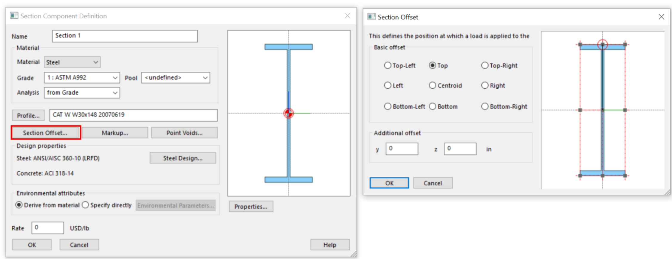
Offsets are visible in the Graphic window when the Section display is switched on

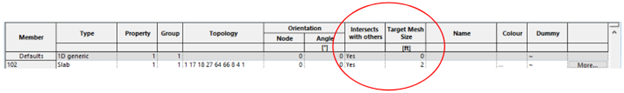
Define 2D member mesh size

1. Go to Explorer pane > Data > Members or click on an existing member graphically and then use the Properties pane to view and modify member properties.

2. In the Members table, under Intersects with others, tick Yes.

   • This ensures the mesh will auto split at beams and other members.

3. Enter an appropriate Target mesh size so that there are enough intermediate nodes between beams or between columns to form a natural mode shape, e.g., 8-10 elements along a beam length and 3-4 elements between secondary beams in a floor bay.

_{Image shows Members table with Target mesh size highlighted}

In the Design layer graphic window, the mesh should be visible and should update automatically each time the Target mesh size value is updated.

Populate the Analysis layer from the Design layer

In the top toolbar, select Model > Coordination tools > Create elements from members.

_{Image shows Create elements from members toolbar option highlighted}

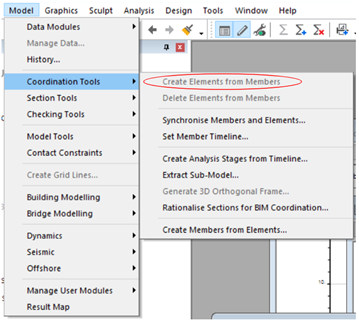
By creating elements from members, this ensures that all beam elements are sub-meshed consistently with the 2D element mesh.

2. Add loading

When applying loading to your model, only consider loads that are relevant to vibration analysis. This will depend on the specific design guide being followed and its recommendations.

• Typically, this includes minimum credible dead load (self-weight and superimposed dead load).
• Sometimes a minimum live load is also allowed by the design guide being followed.

Note: It is important to not overestimate loads as they are considered as mass in the analysis. A higher mass generally results in a lower vibration response, while a lower mass is conservative for a vibration response.

Note: It is not necessary to create Gravity loading to represent the structure’s self-weight if the materials used in analysis have non-zero density. Self-weight loading is calculated automatically for modal analysis.

3. Assign global supports

To assign a global support use the Select nodes tool (keyboard shortcut N) to click on a node and edit its Restraint in the Properties pane.

Global supports are recommended for:

1. Tops of columns that extend above the floor

   • End fixities are user defined. They should capture the most realistic stiffness of the columns in the structure.

2. Interior partitions

   • Where interior partition types and locations are known, global supports such as verical z restraints or spring restraints may be included.
   • Alternatively, explicitly modelled shell or plane stress elements may be included.
   • Ensure these choices are consistent with the design assumptions.

3. Slab edges

   • Partial floor model: the user can rotationally fix the edge of the slab nodes in the slab out-of-plane bending direction to represent bending fixity of the continuous slab not modelled.
   • Full floor model: for an exterior slab where a façade exists, the user can add vertical z restraints to capture vertical stiffness.

4. Base of columns that extend below the floor

   • End fixities are user defined. They should capture the most realistic stiffness of the columns in the structure.

Add slab edge horizontal restraints without inducing membrane action

Slab edge horizontal restraints are useful for providing global horizontal stability, to avoid activating unwanted horizontal modes.

Take care not to over-restrain the floor slab horizontally which can result in unrealistic membrane forces in the floor. For example, this can occur if two opposite sides of a floor slab have their edges restrained in the same horizontal direction.

To view restraints, click the Label restraints icon

Select the Plan view to see edge restraints

4. Run a static analysis

1. Select the New analysis task icon

2. In the Analysis wizard tick Static, then Next.

3. Click Add to select your analysis case, then Finish.

Use these results to check for stability and troubleshoot as necessary to make sure the model runs without errors.

5. Run a dynamic modal analysis

1. In the Data tab of the Explorer pane go to Tasks and cases > Analysis tasks.

_{Image shows Analysis tasks highlighted on Explorer pane}

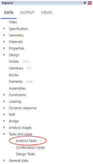
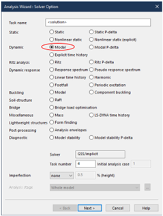
2. Right click and select New analysis task.

_{Image shows New analysis task highlighted in toolbar menu}

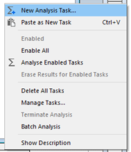
3. Click Modal then Next.

_{Image shows New analysis wizard with Modal highlighted}

4. Set the number of modes.
   • This is iterative. In this example, we have started with one, to check the fundamental frequency. You can add more modes later.
5. Under Mass option tick Lump mass at nodes.
   • This automatically includes the modelled structure’s self-weight based on material densities and element cross sectional areas.
6. Under Mass derived from loads, select or create a load combination that includes all relevant superimposed mass (superimposed dead load and/or live load).
   • Tick z for the Direction.
   • Set the Scale factor to 1.
   • Click Next.

Note: This is only for superimposed loads (not structural self-weight)

7. Tick Analyse then Finish to run the modal analysis.
   • Check the Analysis report for warnings or errors.

For further guidance on modal dynamic analysis in GSA, visit our references entry.

6. Refine the number of modes

1. In the Output tab of the Explorer pane go to: Global results > Dynamic summary. Check the frequency of the lowest mode and highest mode.

2. Re-open the Dynamic analysis task from the Analysis tasks that was created in Step 5 and update the number of modes if necessary.

   • There should be enough modes in the dynamic analysis so that the highest mode has a frequency of >15Hz or twice the natural frequency of the lowest relevant vibration mode, whichever is higher.

3. To specify an upper frequency cut-off, in the Modal analysis task wizard, select Upper from the Frequency cut-offs dropdown, then enter the desired value.

   • This will force the modal analysis to stop calculating results after the cut-off frequency. The last mode calculated will have a frequency lower than the cut-off value to make sure that the number of modes is sufficiently high to capture the highest required frequency.

7. Check mode shapes

1. Above the Graphic window select your modal analysis from the Cases dropdown.

2. Click on the Deformed image icon

3. In the Contours tab of the Properties panel, tick to expand 2D results > 2D displacements > Resolved translation.

Your mode sizes will now be visible. To check if you have enough modes to cover the floorplate:

4. In the Data tab of the Explorer pane select Tasks and cases > Combination case.

5. Create an envelope of all modes. View this envelope in the graphic window to see the distribution of all modes across the floorplate. Un-tick the deformed image icon for a cleaner visual.

8. Create a footfall analysis task

1. In the Data tab of the Explorer pane go to Tasks and cases > Analysis tasks > New analysis task.

2. In the Analysis wizard check Footfall in the Dynamic response, then Next.

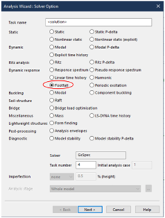
3. Under the Modal analysis task dropdown, select the modal analysis you have just created.

4. Then, define your Excitation method, Response nodes and Excitation nodes as appropriate.

Note: In some cases, only certain nodes should be considered as excitation nodes, while response results are desired at other nodes. E.g., if a hallway is the source of the footfall response across an entire floorplate, only the hallway nodes should be selected as excitation nodes, while all nodes would be response nodes. This can be done by selecting the desired nodes and saving them as a list for easy reference.

5. Number of footfalls: GSA defaults to 100 which is usually conservative.

   • Refine as appropriate, e.g., the number of steps a person can realistically take across a region that excites the primary active mode shape.
   • see step 10 for more detailed information.

6. Walker: Enter the average weight of the expected walker.

7. Direction of responses: As appropriate, typically Z (vertical) in the GSA global axis.

8. Frequency weighting curve: Select whichever option is most appropriate for the analysis, or create your own custom curve.

9. Excitation forces (DLFs): Select whichever option is most appropriate for the analysis or create your own custom curve.

10. Walking frequency (Hz): This will auto-populate depending on the above selection. This can be modified as appropriate for the analysis.

11. Click Next.

12. Damping option: Select whichever option is most appropriate for the analysis.

    • If Constant damping is selected, enter the damping % that is most appropriate for the structure.

13. Click Next then Finish to run footfall analysis.

Further guidance on footfall analysis parameters is available in our references entry.

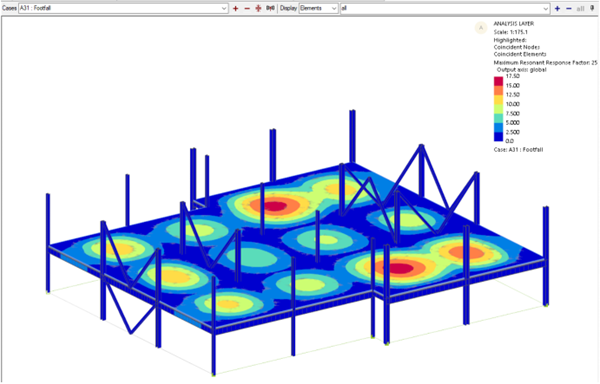
9. Viewing footfall results

1. Above the Graphic window select footfall from the Cases dropdown.

_{Image shows the Cases dropdown menu with a footfall case highlighted}

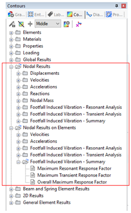
2. In the Contours tab of the Properties panel expand Nodal results or Nodal results on elements to see various types of footfall results displayed graphically.

_{Image shows the Properties panel with Nodal results highlighted}

_{Image shows a plan view of a floor model with **Overall maximum response factor** contoured on the nodes}

_{Image shows a plan view of a floor model with **Overall maximum response factor** contoured on the elements}

_{Image shows an isometric view of a floor model with **Overall maximum response factor** contoured on the elements}

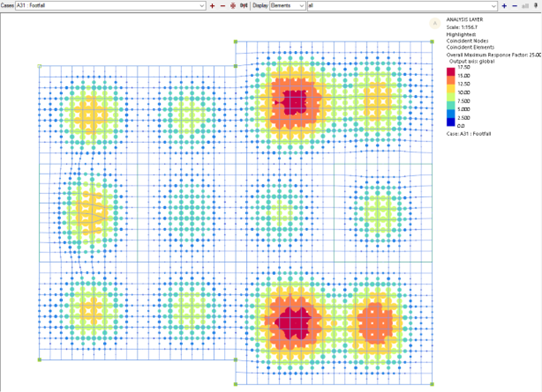
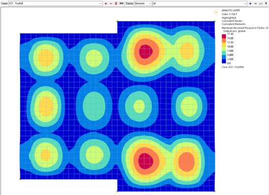
Note: You can save graphic views for easier access.

Chart views

1. In the top toolbar select Views > New chart view > Footfall analysis.

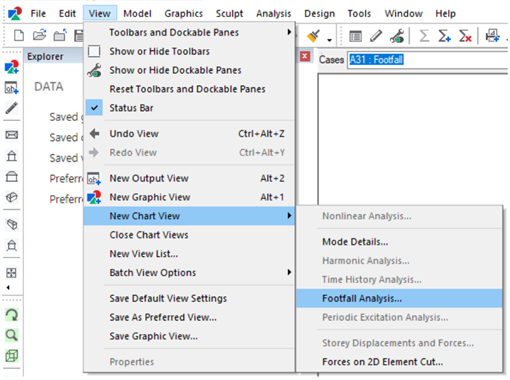
2. Select your chart types from the checklist. Two useful chart types are highlighted below:

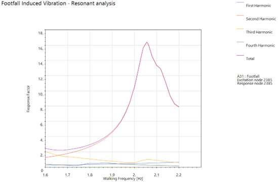
Response factor vs. walking frequency: Shows the response factor for a given node vs. the walking excitation frequency at various harmonics of vibration. Can be used to understand a given node’s sensitivity to different walking frequencies and whether changing the lower and upper bounds of the walking frequency will change the peak response.

_{Image shows a Response factor v. walking frequency chart for node 2385 in an example model. This chart shows that the peak resonant response for this node occurs at a walking frequency of 2.05 Hz}

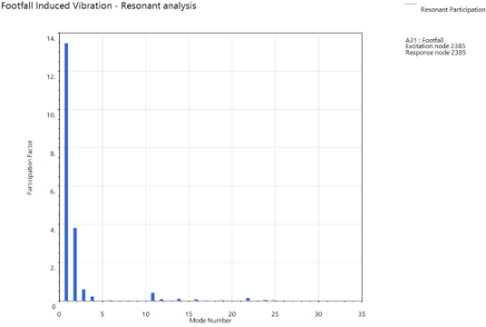
Participation factor vs. modes: Shows each mode’s relative participation factor for a given node. Useful for understanding which modes contribute the most to the footfall vibration response of any given node.

_{Image shows a Participation factor v. modes: resonant chart for node 2385 in an example model. This chart shows that this mode's resonant response is governed by the structure's first mode of vibration.}

3. Select your relevant task from the Footfall analysis task dropdown.

4. Enter values for Response node and Excitation node.

5. Click Ok to view the chart.

10. Refine footfall analysis as needed.

The footfall contours and charts can be used to refine the number of footfalls used in the footfall analysis task.

• Use the results to identify the node with the highest response value.
• Open the Participation factor vs. modes chart for a specific node to identify which mode has the highest participation.
• Switch on the Deflected shape for that mode by clicking the following icon .
• The number of footfalls in the task can be updated to match the number of steps a person can realistically take across that primary mode’s deflected region.
• Re-run the footfall analysis task with the updated number of footfalls.