
# Getting started
# Model creation video
The following video shows how to model, analyse and view results for a simple beam in GSA.
Oasys GSA 10.1 - 1. Model creation from Oasys on Vimeo.
# Step-by-step instructions to create your first GSA model
The following example shows step-by-step instructions on how to model this simple portal frame.

Part 2 of this example will then show how to modify this frame into a concrete structure and how to add a concrete slab.
# GSA overview
GSA allows engineers to create analytical and design models of a structure, then apply loads and actions to the model, analyse the behaviour, and view the analysis results as tabular data, charts, diagrams, or contour plots on the structure.
Once a model exists in GSA it can be edited in the graphics window or the base data can be edited directly via tabular views. The data required depends on the types of analyses being run.
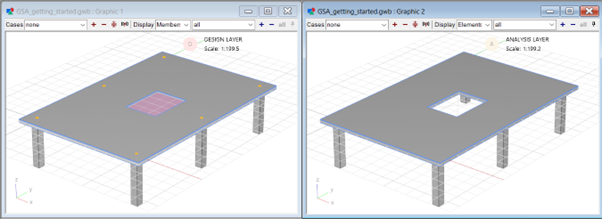
# Layers in GSA
The model exists in two layers: the Analysis layer holds a simplified model of the structure and the Design layer represents the physical structure. Some items, such as nodes, may be mapped between the layers; others may exist only in one layer. The layers can be coordinated with one another using the coordination tools. You are unable to change the analysis data while results exist that depend on that data.
The model can either be imported from a 3D modelling program or created within GSA in the Design layer, the Analysis layer, or both. Wizards assist the initial model creation and subsequent editing.
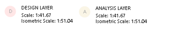
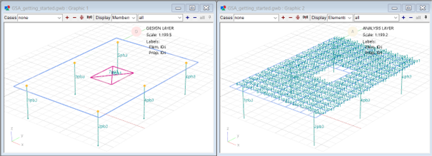
To identify the layer you are currently in, look for the following legend in the top right corner of the graphics window:
To change layers, right click anywhere in the window, and select Switch layer.
You can also use the keyboard shortcut Ctrl+Alt+D.
# Key graphics symbols
| Syntax | As described in this guide | Function |
|---|---|---|
 | Purple square | Selected item |
 | Blue dot | Node |
 | Red dot | Unused node |
 | Yellow dot | Node where members intersect |
 | Red square | Nearest node |
 | Red arrow | Element axis |
 | Grey arrow line(s) | Element or member present on the other layer but not on the current one. Undeformed geometry (if Deformed image is active). |
# Setting up a new model
# Create a new model
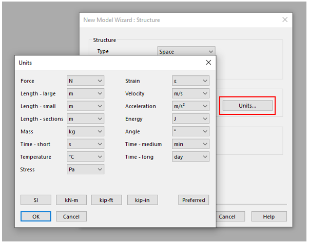
Open GSA and select New model wizard. Alternatively, if you already have a model open, go to File > New from the top menu, (or click Ctrl+N) to bring up the New model wizard.
Name your project and click Next.
Set up Units as appropriate then click Next.
The next screen allows you to specify design codes, material grades, and sections.
# Adding codes, grades and sections
You should now see the New model wizard: Properties:
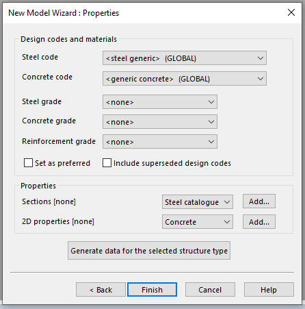
Use the drop down fields to select steel and concrete design codes and grades.
# Adding a steel catalogue
In the properties window, select Steel catalogue > Add.
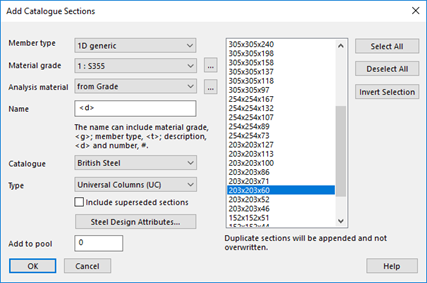
This will bring up the Add catalogue sections dialogue box. The material grade you chose in the previous section will be selected automatically. The analysis material will be set to 'from Grade'.
Set the Name to '<d>' (if it is not already) to use the section description as the section name in your model.
Select your catalogue, and type, and choose from the drop down options.
Then select your section to add.
Click OK to add the section.
Note: Hold the Ctrl key to add multiple sections from the catalogue.
The example below uses British Steel as the catalogue, Universal Columns (UC) as the type and a section of 203x203x60.
You will be taken back to the New model wizard: Properties window. To continue adding catalogue sections, (e.g. for the beam section in the example) repeat steps 1-6 above.
Click Finish to exit the Wizard and start work on your model.
# Creating nodes and 1D members
This section describes how to add nodes to your model and create 1D elements by:
Extruding them from the nodes
Sketching them in the graphics window
# Add support nodes
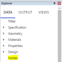
- Go to Explorer pane > Data > Nodes to open the nodes data table.
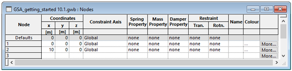
Set the first node at (0,0,0).
Click the first cell and press the Enter key
 to copy all default values from the line above:
In the example below, we have entered '10' as the x coordinate for row 2, then hit Enter to copy all subsequent values in the line above.
Tip: To enlarge the font size in the table. Click Ctrl then scroll up using your mouse wheel.
- In your graphic view, you should now see your nodes on the grid, represented as red dots. Select the Plan tool:
 or press P to change your plan view:
# Setting column type
From the Design layer, select the Entities tool:

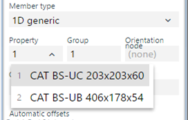
This will bring up the Member properties pane. Press v to show the section of the item you are about to create:
Type E to select members.
The property will be set to '1'. The columns you draw will use the first section defined in the section library.
Under the property drop down, the category codes you have just set up will be visible.
# Creating columns by extrusion
To begin, change the graphic view. Click the Isometric
 (keyboard shortcut i) or Perspective view tool
  (keyboard shortcut k)
Click the Nodes selection tool:
 or use keyboard shortcut n.
Drag or click to select the two nodes you have created. They will show as a purple square:

In the top menu, go to Sculpt > Extrude selection.
In the extrude dialogue box, select your extrusion axis (the default is z).
Add the number of increments and increment length.
Tick Include 1D members along extrusion:
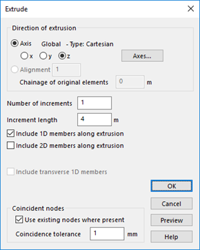
Click Preview to check your elements.
Click OK. Columns are displayed in the graphics window.
# Inspecting elements in the graphics window
The Resize to fit tool changes the graphic view:

From here, you can click and drag the right mouse button to rotate the view.
The Section display tool gives a 3D view of your columns:

Use the Select elements/members tool to select a column and view its properties:

These are displayed in the Messages pane (usually found at the bottom of the graphic window) and Properties pane (typically on the right).
# Creating a beam by sculpting
Select the Add entities tool:
or use keyboard shortcut n.Return to the Member property pane. If you have set up a beam, in the 'property' drop down, change the value to '2' to use the beam section.
Click on the node at the top of one of your columns. A line representing the beam you are about to draw will appear.
Click the node at the top of the other column to complete the beam.
# Setting restraints
Click the Node select icon:
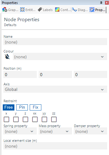
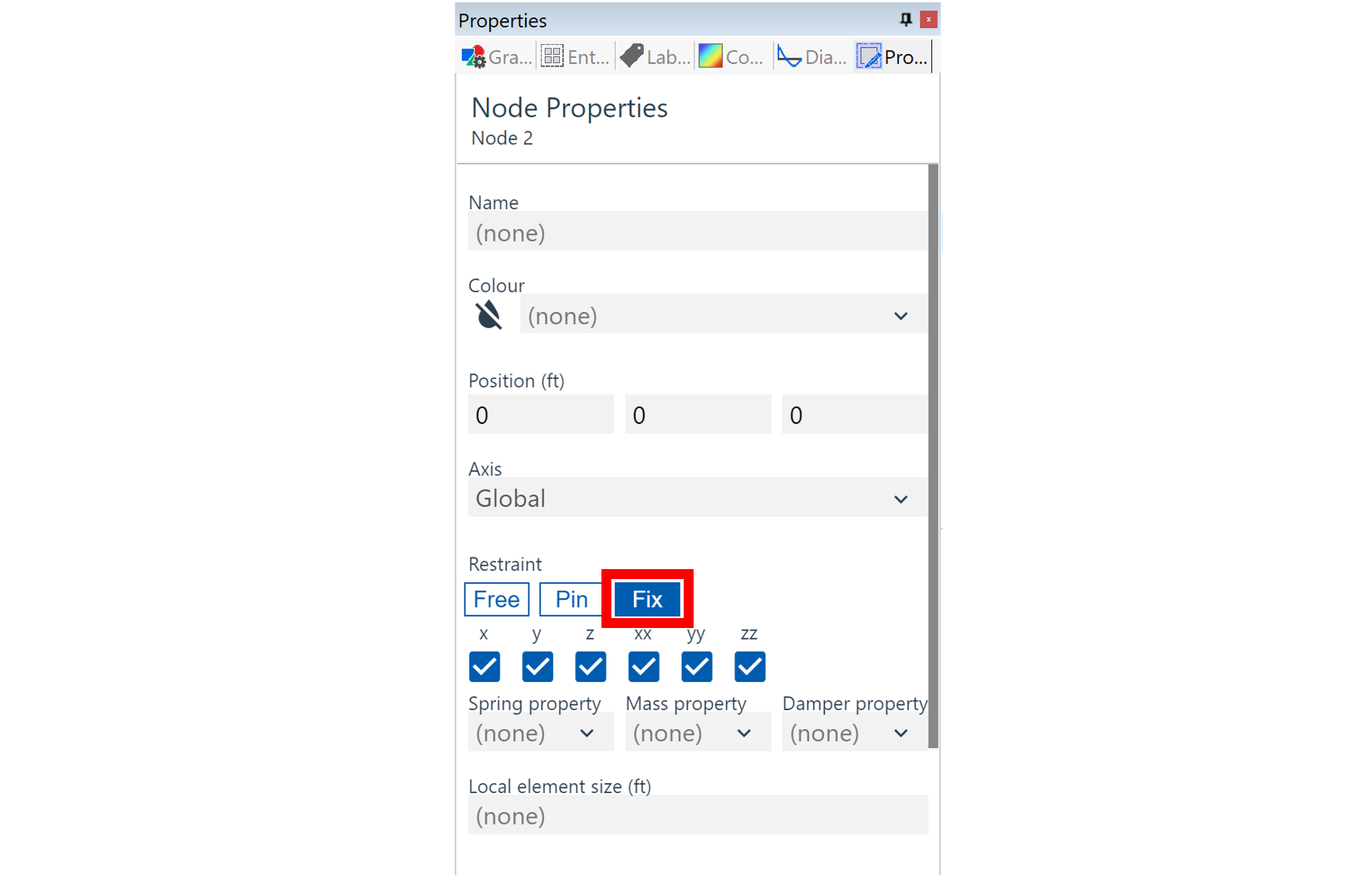
Select the nodes at the bottom the columns to display the Nodes properties pane.
Go to Restraints > Fix to constrain the nodes.
- Select the Label restraints tool to show restraints in the graphics window:

# Applying node and beam loads
This section explains how to create analysis elements and apply loads to the structure. It also shows you how to:
- Mesh the model
- Select items in the graphics window to use in a data table
- Change units using the status bar
- Identify beam ends and apply a load at a specific distance from the end
- Display loads
# Mesh the model
Since we started in the Design layer, we'll need to create the elements on the Analysis layer:
Go to the top menu. Select Model > Coordination tools > Create elements from members.
A dialogue box will appear. Set the member list to All, and press OK.
To continue working with elements in the Analysis layer, you'll need to switch layers.
# Adding self weight loads
Go to Explorer pane > Data > Loading > Gravity loading.
Click the first cell of row 1. Press Enter to copy the default row.
Note: This will calculate the self-weight based on the material density and element volume.

# Creating a lateral load on a node
- Select the node at (0, 0, 4) and press Ctrl+C to copy the selection.
Note: The node coordinates and other settings will appear in the Properties pane.
Go to Explorer pane > Data > Loading > Nodal loading > Node loads to open the node loads table.
Select the first nodes cell on row 1, then press Ctrl+V to paste the node you have selected.
Set the load case to '2' and change the direction of the load to 'x'. Set your value, e.g., 2kN.
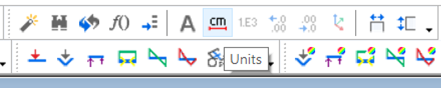
Tip: You can change the unit of your values via the units button in the top toolbar:
# Creating a vertical load on a beam
Click the Select elements tool:
or use keyboard shortcut E, select your cross-beam and click Ctrl+C to copy:Go to Explorer pane > Data > Loading > Beam loading > Beam loads to open the beam loads table.
Use Ctrl+V to paste the selected beam into the row 1 beams cell.
Set the load case to '2' and change the type of the load to point.
Change position 1 of the load, e.g., 2m. This distance is measured in the +ve direction from End 1.
Change the value of the load, e.g., -5kN in the z direction.
# Display loads in the graphics window
Go to the cases dropdown at the top of the graphics window and select L2.
Click the Loads diagram tool to display the loads:

The node and beam loads will be displayed as purple arrows.
# Displaying element axes and flipping elements in the graphics window
If your point load appears towards the wrong end of the beam, you can either move it in the Beam loads table, or you can flip the beam:
- Click the Label element x-axis tool to show the directions of the beams and columns:

Small red cones are drawn on the elements to indicate the local x-axis.
In Element select mode, (E on your keyboard), select your beam.
In the top menu go to Sculpt > Flip elements.
The x-axis arrow will change direction and the point load will move to the other end of the beam.
# Running a simple static analysis
After creating a load case, you can now run a static analysis, and view your results as a table or in the graphics window.
Select the Analyse all icon:

Your analysis is detailed in a report window.
Note: You can view this at any time in Reports tab of the Messages pane.
Return to the graphics window. In the cases drop down select the Analysis case option.
Click the Deformed image icon to show the deformed shape:

bending moments are visible via the Bending moment tool: 
Other common results options are available to view in the diagrams toolbar:

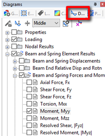
- Go to the Diagrams tab of the Properties pane to access all of the available view options:
# Displaying results as a data table
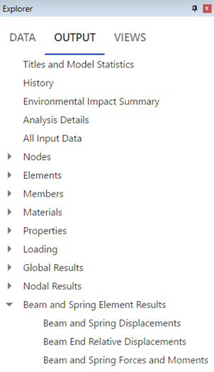
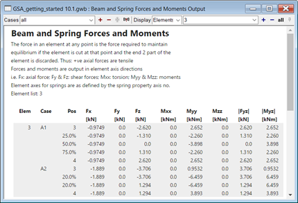
- Go to Explorer pane > Output > Beam and spring element results > Beam and spring forces and moments:
- This will open a table of results. Select Elements in the drop down at the top of the window. Type '3' to show forces on the cross-beam.
# Running a more complex analysis
To run a more complex analysis you need to set up the specific analysis parameters.
Go to Explorer pane > Data > Tasks and cases > Analysis tasks.
Click the New analysis task icon:

This will open the Analysis wizard.
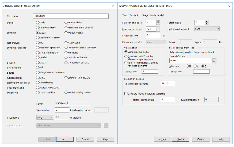
Select the Modal option to define the parameters that control the modal analysis, then Next:
In the next window, set your number of modes, but leave the other parameters unchanged, then click Next:
You have now set up modal analysis, and GSA will run the dynamic analysis.
In the graphics window, go to the Cases drop down and select the analysis case labelled Mode.
Click the Deformed image icon to show the deformed shape:
And the Animate tool to animate the mode shape:

Node: If you cannot see the deformed shape, use the Isometric or Perspective tools to rotate the view:
# Modifying the model
This section shows you how to create a concrete section, assign it to existing members and duplicate existing members.
# Defining concrete sections
You can create different material properties for your Analysis and Design layers. If you have code materials for design, you can derive the analysis properties from them.
When defining sections for columns and beams, you can set which properties you will use. This section shows how to create a 600 x 600 rectangular concrete section.
Go to Explorer pane > Data > Properties > Section Library.
In the next empty row of the table, click the first cell, then the Wizard icon:

Tip: You can also bring up the wizard by double-clicking the next empty row, or pressing Ctrl+W.
In the Name field type '600 x 600'.
Change the Material to concrete.
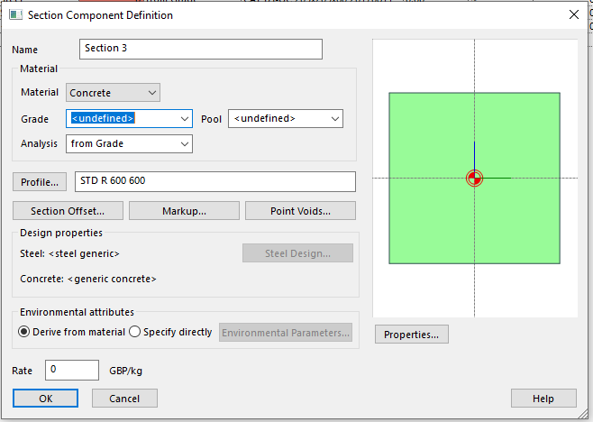
Under Grade, you can either add the grade you defined earlier, or click the More button at the end of the table, to open the Section component definition box. In the Grade drop down, select Add code material.
Return to the section library table. Leave the analysis field as 'from Grade'.
Click More > Section component definition > Profile and tick 'Rectangular'.
Click Next and define the profile as '600 x 600':
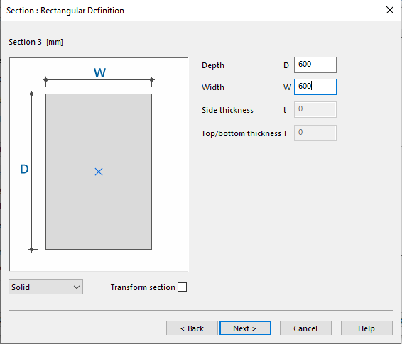
- Click Next and Finish.
The profile definition STD R 600 600 will appear in the profile field, with your defined section on the right.
# Converting existing columns to concrete
Before you can make changes to your analysis model, you must delete any existing analysis results. This section shows how to delete the beam and change your existing column sections to the new concrete ones.
Delete your analysis results by clicking the Delete analyses icon:

In the graphic view, change to the Design layer.
Note: If the structure appears grey, check that the Deformed shape icon is switched off:
Click the Y elevation icon:
 or use keyboard shortcut Y:
Press E to enter Element select mode.
Click on the beam, then press Delete.
Click and drag around the columns to select them.
The elements property pane should now be visible. Select the new concrete section in the property drop down list.
Tip: You can also access the properties pane by using ***Right click > Modify (open properties pane)***.
- In the top menu, go to: Model > Coordination tools > Synchronise members and elements to update the Analysis layer elements.
# Duplicating concrete columns
Select your columns in the graphics window. Click the Copy icon to duplicate:
 This will open the Copy elements dialogue box.
Set the number of copies to '2'.
Set the amount to shift 8m in the Y direction.
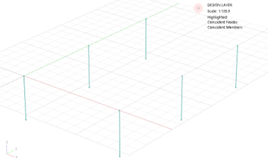
Click OK to return to the graphics window. You should now see six columns. Rotate the view to inspect the columns by right-clicking and dragging.
Click the Section display icon:
to see a 3D view of your columns.
# Creating a 2D member in the design layer
This section shows you how to create a slab with a void, and mesh it using a 2D member. This allows you to create and mesh complex slabs and walls. It covers:
- Creating a grid at a specified elevation
- Defining two 2D members on the current grid
- Specifying that one of the members is a void
- Auto-meshing the slab
Note: This sections assumes that you have six concrete columns. If you are following this guide as a step-by-step tutorial, then you will need to delete any existing analysis results before proceeding.
# Create the grid to draw your slab on
Return to the graphics window. For this example we will begin in the Design layer.
If necessary, click the Draw grid icon:

Right-click a node at the top of one of your columns and select 'Set current grid to this' from the option menu. You will be asked if you wish to create a new grid plane.
Click Yes to create a new grid plane at the top of the columns.
# Draw a 2D member to define the perimeter of your slab
You can now define the shape of your slab by drawing on the plane.
Select the Add entities tool:
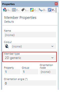
In the Properties pane, set the member type to 2D generic:
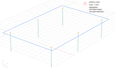
Click on the first corner of your slab. Continue clicking the other corners in either a clockwise or anticlockwise direction.
Finish by clicking back on the first corner, or pressing the Return key.
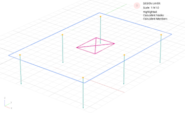
# Define a void cutter member to create a hole in your slab
Select the Add entities tool:
In the Properties pane, set the member type to 2D void cutter.
# Auto-meshing the slab
In the top menu, go to: Model > Coordination Tools > Create Elements from Members.
The members will be meshed into multiple quads and triangles.
# Checking the properties of your slab
- To check your quad definition. Go to: Explorer pane > Data > Elements.
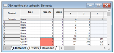
- The property cell is highlighted in red. This shows that you do not have that 2D property defined.
# Setting the properties of your slab
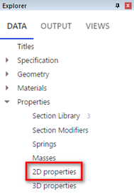
- Go to Explorer pane > Data > Properties > 2D properties:
In the table that opens, confirm the type as shell, and the material as concrete. Check that the grade and analysis values are appropriate.
Set the thickness of your slab to '250mm'.
Close the 2D properties table. Confirm that the red highlighting has gone from the elements table.
# Check your element data in the graphics window
In the graphics window, you should now be able to see that your slab is thicker.
Click the Section display tool to change to a line view of your model.
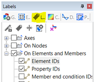
- In the Properties pane, select the Labels tab. Then, tick Element IDs and Property IDs:
- The graphics view will now show the labels, and which associated property has been assigned to each element.
Note: The slab will have a property of PA1. You may need to zoom in to separate the text from the adjacent objects.
- Return to the labels tab of the Properties pane and tick Analysis material IDs.
- Items labelled as m0 shows the analysis material is derived from the material grade.
- Tick Material grade IDs in the Properties pane, to confirm your choices.
- Concrete material grades are prefixed with a c.
- In the labels tab, tick Element axes to confirm that the z-axis (blue line) of your slab is pointing upwards. If not go to Sculpt > Flip elements to correct it.
# Applying a load to the slab
You can apply loads to individual elements, to elements with certain properties, or you can apply a grid load across all the elements on the plane. This section describes how to apply loads using property references.
# Add loads to your slab
To apply a simple load across the whole slab:
Go to Explorer pane > Data > Loading > 2D element loading > Face loads
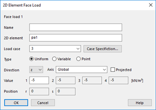
Double click the first cell to bring up the 2D element face load wizard.
In the 2D element field enter 'PA1'.
Set the load case to '3'.
Add a load of −5 kN/m2 in the z global direction and click OK.
Return to the graphics window, Analysis layer.
In the cases drop down, select L3, then the Load diagrams icon:
A face load arrow will be displayed in the centre of each 2D element.
# Displaying the slab displacement as a contour
Go to Explorer pane > Data > Tasks and cases > Analysis tasks and select Delete.
Press Analyse all to analyse the load:
This will recreate the static analysis task and add in all the new load cases.
In the graphics window type P on your keyboard to change to a plan view.
In the Properties pane, select the Contours tab:
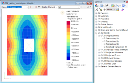
Scroll down until you find the 2D element results options.
- Select an option to display the element displacement results.