Element Stiffness
To generate a stiffness matrix for a curvilinear quadrilateral or
triangular element a new approach must be used. Most finite element
codes used an approach based on isoparametric or similar elements.
In an isoparametric element the element displacements are interpolated
in the same way as the geometry, e.g. a plane stress element. In a
superparametric or degenerate isoparametric element the interpolation on
the geometry is of a higher order than the interpolation of the
displacements, e.g. a plate element. In a subparametric element the
interpolation of the geometry is of a lower order than the interpolation
of the displacements, e.g. an eight noded straight sided quadrilateral
element, where a different geometric interpolation function is used for
the geometry from that for the displacements. The term isoparametric is
often used as a general term to cover all these element types.
For a plane stress problem, we can establish a material matrix C that
relates stress and strain. The displacements in a local coordinate
system are
u={u,v} the strains are
ε={εxx,εyy,γxy} and the stresses are
σ={σxx,σyy,τxy} For an elastic-isotropic material the material matrix is
Cp=1−ν2E⎣⎢⎡1νν121−ν⎦⎥⎤ where E,ν are the Young’s modulus and Poisson’s ratio respectively.
Note that there is an out of plane strain εzz, which we
can ignore as it plays no part in the element formulation.
The strains are defined in terms of the displacements as
εxx=∂x∂uεyy=∂y∂vγxy=∂y∂u+∂x∂v The simplest elements to consider are the 4 noded and 8 noded
quadrilateral elements, of which the 4 noded element can be considered a
simplification of the 8 noded element. A typical 8 noded element is
shown below. The element has an arbitrary local coordinate system based
on the location of the nodes and the element property axis (x,y), and a
natural (curvilinear) coordinate system (r,s) based on the topology of
the nodes.
We can set up interpolation functions to interpolate the geometry as
follows
xs(r,s)=i∑hixm,i where the hi are the interpolation functions defined below.
These interpolation functions are chosen so that
hi={10}when node is{i=i} As the elements are isoparametric we use the same interpolation function
for the displacements so the displacement in the element is related to
the nodal displacements by
us(r,s)=i∑hium,i To evaluate the stiffness matrix we need the strain-displacement
transformation matrix. The element displacements are obtained in terms
of derivatives of the element displacements with respect to the local
coordinate system (x,y). Because the elements displacements are in the
natural coordinate system (r,s) we need to relate the derivatives in
the local coordinate system to those in the natural coordinate system.
We can write an equation for the derivative with respect to x in terms
of derivatives with respect to (r,s)
∂x∂=∂r∂∂x∂r+∂s∂∂x∂s to establish these derivatives we use the chain rule to set up the
following relationship
[∂r∂∂s∂]=[∂r∂x∂s∂x∂r∂y∂s∂y][∂x∂∂y∂] or in matrix notation
∂r∂=J∂x∂ where J is the Jacobian operator relating natural coordinate
derivatives to local coordinate derivatives. Given that we know x and y
in terms of the interpolation functions the Jacobian operator is easily
found
∂x∂=J−1∂r∂ This requires that the inverse of the Jacobian exist, which requires
that there is a one to one correspondence between natural and local
coordinates. This will be the case provided the element is not grossly
distorted from a square and that it does not fold back on itself.
We can then evaluate
∂x∂u,∂y∂u,∂x∂v,∂y∂v and thus we can construct the strain-displacement transformation matrix,
B
ε=Bu where u is the vector of nodal displacements. The element
stiffness corresponding to the local element degrees of freedom is then
K=∫VBTCBdV The elements of B are functions of the natural coordinate
system, (r,s). Therefore the volume integration extends over the
natural coordinate volume so the volume differential needs to be written
in terms of the natural coordinates
dV=detJdrds The volume integral is not normally amenable to an explicit integration
so normally a numerical integration technique is used. The integral can
be written
K=∬r,sFdrds where
F=BTCBdetJ and the integral is performed in the natural coordinate system of the
element. This is convenient as the limits of the integration are then
±1. The stiffness can then be calculated
K=∑αijFij where the matrix F is evaluated at the Gaussian integration
points (ri,si) and αij are Gaussian
weights.
In a similar way the mass matrix and the load vectors are established.
M=∫VρHTHdV rb=∫VHTfbdV rs=∫SHsTfsdS ri=∫VBTτidV where H is a matrix of interpolation functions and
rb,rs,ri, are the body force
vector, surface force vector and initial stress vector respectively.
Layered shell
Stiffness in a rotated axis
For an isotropic material the properties are invariant with direction so any difference between element and material axis is not relevant.
For an orthotropic material this will make an impact on the element stiffness in this case the material matrix should be rotated from
the material axis, m, to the element axis, e, before building the stiffness matrix.
Ce=RtCmR
Stiffness
The stiffness of a composite (layered) shell is calculated from a stack of linked shells representing each layer. For each layer
fi=Kiui If the offset of the layer is z then the relationship between the layer and the centre of the elements is given by
\begin{align} u_{x,i} &= u_x + \theta_y z_i \\ u_{y,i} &= u_y - \theta_x z_i \\ u_{z,i} &= u_z \\ \theta_{x,i} &= \theta_x \\ \theta_{y,i} &= \theta_y \\ \theta_{z,i} &= \theta_z \\ \end{align}
The matrix representing this transformation is
Ti=⎣⎢⎢⎢⎢⎢⎢⎢⎡111−zi1zi11⎦⎥⎥⎥⎥⎥⎥⎥⎤ So for a layer related to the centre of the element
f~i=(TiTKiTi)u So integrating over the layers
K=i∑(TiTKiTi) Geometric stiffness matrix of shell element
The geometric stiffness matrix is calculated from:
Kg=∫AGTNGdA=∬r,sGTNGdetJdrds where
N=[NxNyxNxyNy] With (Nx,Ny,Nxy) are the in-plane forces of the
shell element in x, y and xy shear directions respectively.
G=[G1G2…Gn] and n is the number of nodes of the elements
Gi=[0000∂x∂hi∂y∂hi000000] 2D Plate Elements
The formulation of 2D plate and shell elements considers both in-plane
and transverse (out-of-plane) displacements. Following Mindlin-Reissner
plate theory, in addition to the bending strains we consider the effect
of transverse shear strain in our complete expression for the element
strain
{γxzγyz}={∂x∂w−βx∂y∂w−βy} where w is the out-of-plane displacement and β is introduced as an
independent variable to express the section rotations (i.e. rotations of
the transverse normals about the local x and y axes).
We can define separate material matrices Cb and
Cs that relate stress and strain for the pure bending and
shear strains respectively and so the pure bending moments and shear
forces can be written
⎩⎪⎨⎪⎧σxxσyyτxy⎭⎪⎬⎪⎫=−zCb⎩⎪⎪⎨⎪⎪⎧∂x∂βx∂y∂βy∂y∂βx+∂x∂βy⎭⎪⎪⎬⎪⎪⎫ and
{τxzτyz}=Cs{∂x∂w−βx∂y∂w−βy} respectively.
In this way we can then express the local element stiffness matrix as a
summation of the in-plane and out-of-plane stiffness’s
K=∫V(BκTCbBκ+BγTCsBγ)dV where Bκ and Bγ represent the
strain-displacement transforms for the bending and shear components
respectively.
While brief, this outlines the basic approach to the Mindlin-Reissner 2D
element stiffness formulation. In GSA we label this concisely as the
Mindlin formulation.
We find that the Mindlin formulation is an effective approach for 2D
parabolic elements where the 8-noded element accommodates sufficient
terms in the stiffness matrix to sufficiently define the behaviour of
the element numerically. However the same formulation defined over a
linear element becomes noticeably more problematic where the absence of
available terms in our 4-noded stiffness matrix leads to numerical
difficulties in expressing the same element behaviour. Specifically we
find a difficulty in attempting to represent the transverse shear strain
terms. Analytically as before we can express the transverse shear strain
as
{γxzγyz}={∂x∂w−βx∂y∂w−βy} although numerically, the difference in the order of terms for the shear
strain may lead to artificial stiffening of the element where the shear
terms are numerically constrained from approaching zero. See reference 1
in the bibliography for further information. This restriction would be
particularly noticeable where the thickness of the plate is small.
A widely practiced remedy is to under-integrate the shear term and while
effective, its use is at the cost of reduced accuracy and stability for
the element. The problem of stability alone is often of greatest concern
where the phenomenon of hourglassing can become apparent in elements
where the thickness to length ratio is large.
An alternative formulation was put forward by Bathe and Dvorkin and has
been found to be especially effective at resolving these difficulties.
The formulation is extendable to higher order elements although we find
the approach is most effective when resolving the difficulties most
apparent in linear elements. The formulation is based upon the theory of
Mixed Interpolated Tensoral Components (MITC). For the pure
displacement-based Mindlin formulation we use the independent variables
wβ=i=1∑nhiTwi=i=1∑nhiTθi where Bathe now introduces a separate independent variable to represent
the transverse shear term
γ=i=1∑nhi∗TγPi We use hi∗ to represent an additional set of
interpolation functions for our new variable γ which we find by a
direct evaluation of the shear strain at points Pi, that is
γPi=(∂x∂w−β)Pi For a linear 2D element we obtain direct values for the shear strain at
four points A, B, C, D on the element and so we evaluate the
displacement and section rotations at these points through direct
interpolation.

We can then construct the interpolations
γrzγsz=21(1+s)γrzA+21(1−s)γrzC=21(1+r)γszD+21(1−r)γszB using direct values for the shear strains obtained at the four points.
This replaces our original expression for the shear terms and we
continue to construct the local stiffness matrix as normal in a similar
approach as before in 2D isoparametric elements. It is lastly worthwhile
to note that the interpolation above assumes our element is in the
isoparametric coordinate system. Further transformations are necessary
to interpolate the shear strains directly through an arbitrary element
in local space. Indeed, when this is done the element shows considerably
improved predicative capabilities for distorted elements.
Element shape functions
The element shape functions for 2D elements are
u(r,s)=i∑hiui These are for the different element shapes
Tri-3
h1h2h3=1−r−s=r=s Quad-4
h1h2h3h4=41(1−r)(1−s)=41(1+r)(1−s)=41(1+r)(1+s)=41(1−r)(1+s) Tri-6
h1h2h3h1h2h3=1−r−s−21h4−21h6=r−21h4−21h5=s−21h5−21h6=4r(1−r−s)=4rs=4s(1−r−s) Quad-8
h1h2h3h4h5h6h7h8=41(1−r)(1−s)−21h5−21h8=41(1+r)(1−s)−21h5−21h6=41(1+r)(1+s)−21h6−21h7=41(1−r)(1+s)−21h7−21h8=41(1−r2)(1−s)=41(1+r)(1−s2)=41(1−r2)(1+s)=41(1−r)(1−s2) 2D Element Shape Checks
A number of element checks are carried out by GSA prior to a GSS
analysis. Other analysis programs may have different limits but the same
principles apply. For GSS the following warnings, severe warnings and
errors are produced.
Triangle
| Warning | Severe warning | Error |
|---|
| 5<rmax≤15 | rmax>15 | |
| 15≤θmin<30 | θmin<15 | |
| 150≤θmax≤165 | | θmax>165 |
Quad
| Warning | Severe warning | Error |
|---|
| 5<rmax≤15 | rmax>15 | |
| 25≤θmin<45 | θmin<25 | |
| 135≤θmax≤155 | | θmax>155 |
| 0.00001<hmax≤0.01 | hmax>0.01 | |
where
rmax longest side / shortest side
θmin minimum angle
θmax maximum angle
hmax distance out of the plane of the element of edge 1 / longest
side
Notes:
The distance out of plane of edge 1 is calculated as hmax
hmax=smaxn⋅(c2−c1) Where n is the element normal, c1, c2
are the coordinates of the first and second corner nodes and smax
is the length of the longest side of the element.
Mid-side node locations not checked but should be approximately halfway
along edge.
No check on ratio thickness/shortest side.
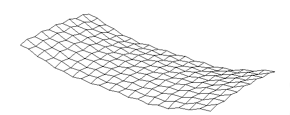
Hourglassing
When Quad 4 elements with the Mindlin formulation are used in bending it
is possible to encounter hourglassing problems. This is a problem that
arises with under-integrated elements where there are insufficient
stiffness terms to fully represent the stiffness of the element. The
problem is noticeable in the results by an hourglass pattern in the mesh
as shown below.
This problem is avoided using the MITC formulation for Quad 4 elements.
This formulation uses a separate interpolation method for the transverse
shear strains and provides considerably greater stability than the
original Mindlin method. The original Mindlin method is kept in GSA for
compatibility with previous models although for new models the MITC
formulation is recommended.
Alternatively when parabolic accuracy is required Quad 8 elements are
recommended. These also formulate elements that are still stiff in all
modes of deformation, even when under-integrated.
3D Element
The element shape functions for 2D elements are
u(r,s,t)=i∑hiui These are for the different element shapes
Tetra-4
h1h2h3h4=81(1−r)(1−s)(1−t)=81(1+r)(1−s)(1−t)=41(1+s)(1−t)=21(1+t) Pyramid-5
h1h2h3h4h5=81(1−r)(1−s)(1−t)=81(1+r)(1−s)(1−t)=81(1+r)(1+s)(1−t)=81(1−r)(1+s)(1−t)=21(1+t) Wedge-6
h1h2h3h4h5h6=81(1−r)(1−s)(1−t)=81(1+r)(1−s)(1−t)=41(1+s)(1−t)=81(1−r)(1−s)(1+t)=81(1+r)(1−s)(1+t)=41(1+s)(1+t) Brick-8
h1h2h3h4h5h6h7h8=81(1−r)(1−s)(1−t)=81(1+r)(1−s)(1−t)=81(1+r)(1+s)(1−t)=81(1−r)(1+s)(1−t)=81(1−r)(1−s)(1+t)=81(1+r)(1−s)(1+t)=81(1+r)(1+s)(1+t)=81(1−r)(1+s)(1+t) The stiffness matrix for brick elements is obtained using selective
reduced integration to alleviate volumetric locking. The
Bˉ approach has been implemented in GSA where the
strain-displacement matrix is split into dilatational and deviatoric
parts7 and then the dilatational part of matrix is replaced with
improved dilatational component. The strain-displacement matrix for
brick elements is given by
B=⎣⎢⎢⎢⎢⎢⎢⎢⎡B1000B3B20B20B30B100B3B2B10⎦⎥⎥⎥⎥⎥⎥⎥⎤ The dilatational and deviatoric parts of the matrix can be computed
using
BdilBdev=⎣⎢⎢⎢⎢⎢⎢⎢⎡B1B1B1000B2B2B2000B3B3B3000⎦⎥⎥⎥⎥⎥⎥⎥⎤=B−Bdil Bˉ is computed using
BˉBˉdil=Bdev+Bˉdil=31⎣⎢⎢⎢⎢⎢⎢⎢⎡Bˉ1Bˉ1Bˉ1000Bˉ2Bˉ2Bˉ2000Bˉ3Bˉ3Bˉ3000⎦⎥⎥⎥⎥⎥⎥⎥⎤ and
Bˉi=∫dΩ∫BidΩi=1,2 and 3 for i=1,2 and 3, and where ∫dΩ is the volume of
the element.
Link Element
Link elements are different to the other element types in that they
apply a constraint between a pair of nodes. The primary node is the
first node specified in the element topology and this is the node that
is retained in the solution. The other node (the constrained node) is
related back to the primary node.
us=Tum The degrees of freedom at the constrained node that are linked will
depend on the type of link. The link allows the constrained node to be
fixed (where the rotations at the constrained node depend on the
rotation of the primary) or pinned (where the rotations at the
constrained node are independent of the rotation of the primary). The
primary node is always has the rotations linked to the rest of the
structure. The links can act in all directions or be restricted to act
in a plane (xy, yz or zx) where the nodes are rigidly connected for
motion in the plane but are independent for out of plane motion.
The constraint conditions are summarised below:
All directions
⎣⎢⎢⎢⎢⎢⎢⎢⎡1000000100000010000−zyδ00z0−x0δ0−yx000δ⎦⎥⎥⎥⎥⎥⎥⎥⎤ where δ=1/0 if fixed / pinned Plane (xy plane as example)
⎣⎢⎢⎢⎢⎢⎢⎢⎡100000010000000000000000000000−yx000δ⎦⎥⎥⎥⎥⎥⎥⎥⎤ where δ=1/0 if fixed / pinned Loads applied to link elements will be correctly transferred to the
primary degree of freedom as a force + moment so no spurious moments
result.
The inertia properties of a link element can be calculated from the
masses at the nodes attached to the rigid element as follows. The mass
is
m=i∑mi and the coordinates of the centre of mass are
xc=m∑imixiyc=m∑imiyizc=m∑imizi The inertia about the global origin is then
Iˉxx=i∑mi(yi2+zi2)Iˉxy=−i∑mixiyiIˉyy=i∑mi(zi2+xi2)Iˉyz=−i∑miyiziIˉzz=i∑mi(xi2+yi2)Iˉzx=−i∑mizixi and relative to the centre of mass (xc,yc,zc) this is
Ixx=i∑mi((yi−yc)2+(zi−zc)2)Iˉxy=−i∑mi(xi−xc)(yi−yc)Iyy=i∑mi((zi−zc)2+(xi−xc)2)Iˉyz=−i∑mi(yi−yc)(zi−zc)Izz=i∑mi((xi−xc)2+(yi−yc)2)Iˉzx=−i∑mi(zi−zc)(xi−xc) The constraint equations for a link element assume small displacements.
When large displacements are applied to a link element the constraint
equations no longer apply and the links between constrained and primary
get stretched. This effect can be noticeable in a dynamic analysis where
the results are scaled to an artificially large value. When these are
scaled to realistic value this error should be insignificant.
7 Hughes T. J. R. The Finite Element Method – Linear Static and Dynamic Finite Element Analysis, Dover, 2000

