Response Spectrum Analysis

Response Spectrum

The response of a single degree of freedom system mode (frequency $f$, spectral acceleration $a_{spectral}$) is

$$q_{i} = \frac{a_{spectral}}{(2\pi f)^{2}}$$

Modal analysis reduces a complex structure to an equivalent system of single degree of freedom oscillators so this can be applied to the structure as a whole for any selected mode. The response in a given mode $i$ in direction $j$ is

$$\mathbf{x}_{ji} = \Gamma_{ij}\frac{a_{spectral}}{(2\pi f_{i})^{2}}\phi_{i}$$

Where $\Gamma_{ij}$ is the participation factor to account for the direction of excitation. The term

$$\Gamma_{ji}\frac{a_{spectral}}{(2\pi f_{i})^{2}}$$

is the modal multiplier.

For global x and y we use $\Gamma_{x}$ & $\Gamma_{y}$. So for excitation at an angle α we want to use $\Gamma_{\alpha}$. Going back to the definition of the participation factor in x and y directions:

$$\Gamma_{x} = \frac{\phi^{T}\mathbf{Mx}}{\widehat{m}}$$

$$\Gamma_{y} = \frac{\phi^{T}\mathbf{My}}{\widehat{m}}$$

Where x and y corresponds to a rigid body displacement in the respective direction. So the rigid body vector at $\alpha$ is

$$\mathbf{r}_{\alpha} = \mathbf{x}\cos\alpha + \mathbf{y}\sin\alpha$$

And the orthogonal direction $\alpha'$ would have a rigid body vector

$$\mathbf{r}_{\alpha'} = - \mathbf{x}\sin\alpha + \mathbf{y}\cos\alpha$$

This means that for a rotated excitation direction we just need to rotate the participation factors and we don’t need to transform the displacements, etc.

$$\Gamma_{\alpha} = \frac{\phi^{T}\mathbf{Mx}}{\widehat{m}}\cos\alpha + \frac{\phi^{T}\mathbf{My}}{\widehat{m}}\sin\alpha$$

$$\Gamma_{\alpha'} = - \frac{\phi^{T}\mathbf{Mx}}{\widehat{m}}\sin\alpha + \frac{\phi^{T}\mathbf{My}}{\widehat{m}}\cos\alpha$$

or

$$\Gamma_{\alpha} = \Gamma_{x}\cos\alpha + \Gamma_{y}\sin\alpha$$

$$\Gamma_{\alpha'} = - \Gamma_{x}\sin\alpha + \Gamma_{y}\cos\alpha$$

That leaves the only transformation we need being the transformation of global displacements to local for nodes in constraint axes. For these we want to transform modal results from global to local, do the combination and transform combined value from local to global.

The modal responses are then combined using one of several combination methods.

Combinations

The main combination methods are:

ABSSUM

$$x = \sum_{i}^{}\left| x_{i} \right|$$

SRSS

$$x = \sqrt{\sum_{i}^{}{x_{i}}^{2}}$$

CQC$^2$

$$x = \sqrt{\sum_{i}^{}{\sum_{j}^{}{x_{i} \cdot \rho_{ij} \cdot x_{j}}}}$$

where

$$\rho_{ij} = \frac{8\sqrt{\zeta_{i}\zeta_{j}}\left( \zeta_{i} + \beta_{ij}\zeta_{j} \right){\beta_{ij}}^{\frac{3}{2}}}{\left( 1 - {\beta_{ij}}^{2} \right)^{2} + 4\zeta_{i}\zeta_{j}\beta_{ij}\left( 1 + {\beta_{ij}}^{2} \right) + 4\left( {\zeta_{i}}^{2} + {\zeta_{j}}^{2} \right){\beta_{ij}}^{2}}$$

where $\zeta_{i}$ and $\zeta_{j}$ are the damping associated with frequencies $f_{i}$ and $f_{j}$ respectively.

$$\beta_{ij} = \frac{f_{i}}{f_{j}}\quad f_{j} \geq f_{i}$$

If the damping is constant this simplifies to

$$\rho_{ij} = \frac{8\zeta\left( 1 + \beta_{ij} \right){\beta_{ij}}^{\frac{3}{2}}}{\left( 1 - {\beta_{ij}}^{2} \right)^{2} + 4\zeta\beta_{ij}\left( 1 + \beta_{ij} \right)^{2}}$$

Rosenbluth$^3$

$$x = \sqrt{\sum_{i}^{}{\sum_{j}^{}{x_{i} \cdot \rho_{ij} \cdot x_{j}}}}$$

where

$$\rho_{ij} = \frac{\frac{2\sqrt{\zeta_{i}\zeta_{j}}}{\left( \zeta_{i} + \zeta_{j} \right)}}{1 + \left\lbrack \frac{\left( f_{i} - f_{j} \right)}{\left( \zeta_{i}f_{i} + \zeta_{j}f_{j} \right)} \right\rbrack^{2}}$$

CQC3

In SRSS method, the spectra $s_{x},s_{y}$ are applied to 100% on the principal directions. The responses obtained from SRSS combination has equal contributions from all the directions. However, in practice the same ground motion will not occurs in both the direction. Therefore, SRSS yields conservative results.

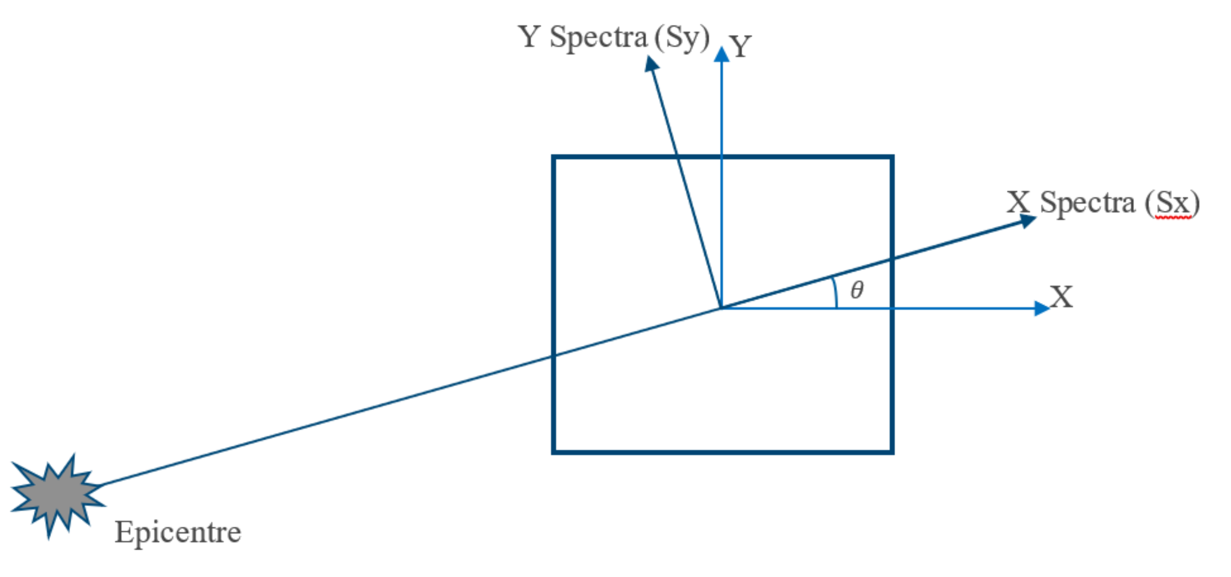
Menun and Der Kiureghian$^4$ (1998) presented the CQC3 combination method for combination of the orthogonal spectrum. Let assume $s_{x},s_{y}$ are the major and minor spectra applied at an arbitrary angle $\theta$ from the structural axis. To simplify the analysis further assume the $s_{y}$ spectra is some fraction of $s_{x}$ spectra.

$$s_{y} = a \times s_{x}$$

The peak response value can be estimated using the fundamental CQC3 equation

$$Q = \left\lbrack {Q_{x}}^{2} + a_{2}{Q_{y}}^{2} - \left( 1 - a^{2} \right)\left( {Q_{x}}^{2} - {Q_{y}}^{2} \right)\sin^{2}\theta + 2\left( 1 - a^{2} \right)Q_{xy}\sin\theta\cos\theta + {Q_{z}}^{2} \right\rbrack^{\frac{1}{2}}$$

where

$${Q_{x}}^{2} = \sum_{i}^{}{\sum_{j}^{}{q_{xi}\rho_{ij}q_{xj}}}$$

$${Q_{y}}^{2} = \sum_{i}^{}{\sum_{j}^{}{q_{yi}\rho_{ij}q_{yj}}}$$

$$Q_{xy} = \sum_{i}^{}{\sum_{j}^{}{q_{xi}\rho_{ij}q_{yj}}}$$

$${Q_{z}}^{2} = \sum_{i}^{}{\sum_{j}^{}{q_{zi}\rho_{ij}q_{zj}}}$$

and $q_{xi},q_{yi}$ are the modal quantities produced by spectrums applied at x and y directions, $q_{zi}$ is the modal value produced by the vertical spectrum and $\theta$ is the arbitrary angle at which the lateral spectra is applied.

Normally, the value of $\theta$ is not known. The critical angle that produces maximum response can be calculated using

$$\theta_{cr} = \frac{1}{2}\tan^{- 1}\left( \frac{2Q_{xy}}{{Q_{x}}^{2} + {Q_{y}}^{2}} \right)$$

And the critical response becomes

$$Q = \left\lbrack {Q_{x}}^{2} + a_{2}{Q_{y}}^{2} - \left( 1 - a^{2} \right)\left( {Q_{x}}^{2} - {Q_{y}}^{2} \right)\sin^{2}\theta_{cr} + 2\left( 1 - a^{2} \right)Q_{xy}\sin\theta_{cr}\cos\theta_{cr} + {Q_{z}}^{2} \right\rbrack^{\frac{1}{2}}$$

If the value of $a = 1$, CQC3 combination reduces to SRSS combination. The peak response value is not dependent on the $\theta$ and the peak response can be estimated using.

$$Q_max=\sqrt{Q_x^2+Q_y^2+Q_z^2}$$

There is no specific guidelines available to choose the value of $a$. Menun and Der Kiureghian presented an example for CQC3 combination with a value ranging from 0.50 to 0.85.

Storey Inertia Forces

The storey inertia forces can be calculated from the storey mass, m, and inertia, I_zz, response spectrum and the modal results. The storey modal translations (u_x,u_y)and rotations (θz) are calculated (see below)

The force and moment for excitation in the i^th direction are then determined from

$$\begin{aligned}f_{x} &= m.s_{code}\sum_{CQC}^{}\left( \Gamma_{i}a_{spec}u_{x} \right)\\ f_{y} &= m.s_{code}\sum_{CQC}^{}\left( \Gamma_{i}a_{spec}u_{y} \right)\\ M_{z} &= I_{zz}.s_{code}\sum_{CQC}^{}\left( \Gamma_{i}a_{spec}\theta_{z} \right)\end{aligned}$$

Where $s_{code}$ is the code scaling factor, $a_{spec}$is the spectral acceleration and $\Gamma_{i}$ the participation factor.

---

$^2$ Wilson, der Kiureghian & Bayo, 'Earthquake Engineering and Structural Dynamics', Vol 9, pp 187-194 (1981)

$^3$ ASCE 4-09 Seismic analysis of safety related nuclear structures and commentary', Chapter 4.0 Analysis of Structures (2009)

$^4$ Menun, C., and A. Der Kiureghian. 1998. “A Replacement for the 30 % Rule for Multicomponent Excitation,” Earthquake Spectra. Vol. 13, Number 1. February.