Individual component buckling
Individual component buckling analysis allows for determining the axial load capacity of a single beam element or a series of beam elements within a structure under normal applied loads.
In this option, the effective length of an element or a chain of compressive beam elements in a structure can be estimated. This is useful for estimating the degree of restraint offered by the whole structure under a particular load condition. This is especially relevant to nonlinear structures where the degree of restraint offered by ties and cables varies with load case.
The program conducts the analysis with all loads applied at 100%, referred to as the first step analysis. If this step converges successfully, indicating good conditioning of the structure, the number of cycles required for convergence under applied loads is recorded as a measure of structural stability. Equilibrium element forces are stored, and a small moment is added to the member under scrutiny to initiate buckling (as buckling typically requires a small disturbance).
The next step is to reanalyse with the resultant element forces and imposed loads from the initial analysis but with a factored axial force in the member under consideration. This is repeated until the member in question buckles.
Buckling is deemed to occur when the analysis fails to converge within five times the number of cycles that achieved the convergence in the first step analysis. In cases of snap-through during the analysis, the buckling load isn't directly provided; however, it can be deduced by plotting a load-deflection curve using data from the report view. If such a curve is not generated, results should be carefully reviewed.
1. Setting up the model
Create a new GSA file or open an existing model. Create members, elements, nodes, restraints, etc. as per usual keeping in mind of the following implications for buckling analysis.
1D elements
Elements specified should not be bars or struts.
Restraints
It is advised to use nodal restraints. As buckling effects are three dimensional, it is not advised to define global restraints on the structure, as this can potentially provide an artificial degree of stiffness to the model. To add nodal restraints, select Nodes and modify supports conditions from Property > Restraints.
Releases
If you want to avoid transferring moments between elements add end releases: Properties > Releases.
Meshing members
In order to capture buckling within a single member it is advisable to mesh it in a way such that there are at least two elements per member.
To change the mesh size, select the member and go to the Properties pane to modify the analysis element size.
To generate analysis elements from the members, use the Create elements from members tool from Model > Coordination tools > Create elements from members or use the toolbar shortcut.
2. Setting up an analysis task
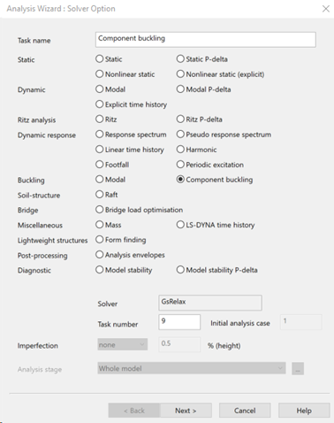
Analysis parameters
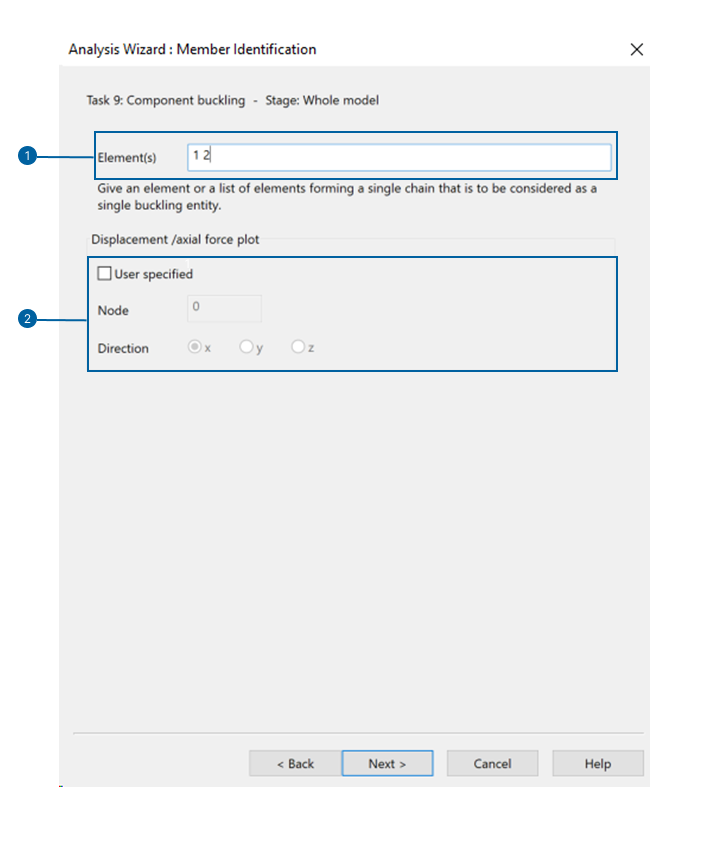
- Element(s): Input a list of beam elements to be investigated for individual component buckling. These must be adjacent elements that represent a single component of concern.
- Displacement / axial force plot: Based on this node a force / deformation graph is generated.
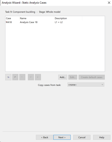
Analysis case
In this case the relationship between load and deformation is no longer linear. For this reason, the load cases must be defined within the analyses and the results cannot be extrapolated later as a linear superposition of the effects of the different loads.
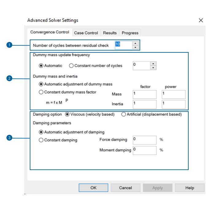
Convergence control
-
Number of cycles to check residuals: The convergence of the solution depends on the magnitude of the residual vector, however, checking the residual takes time so this is not usually calculated at every step.
-
Dummy mass update: A dynamic relaxation solution assigns dummy mass to the nodes which is updated during the solution. In general it is best to leave the updating to the Automatic option, but the user can take control of how frequently this happens. In some cases it may be better not to update the dummy mass, and instead specify a dummy mass factor directly.
-
Damping: Choose between viscous damping (based on the pseudo velocities) or artificial damping (based on displacements). This can be handled automatically, or with a user defined percentage of damping.
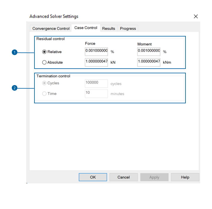
Case control
-
Residual: Set the maximum acceptable out-of-balance conditions. The convergence of the analysis can be adjusted by selecting the Advanced button. This will allow you to adjust the damping and mass, and the frequency at which the dynamic relaxation process is paused to check residuals and recalculate the dummy mass.
-
Termination: Set the maximum number of cycles or the length of time (clock time) for which the analysis should run before terminating.
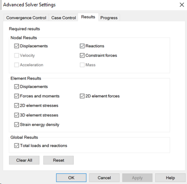
Results
GSA can calculate a large range of results. Because not all these results may be required, selection of particular results to be stored is supported. For an explicit solver these can be selected separately for Full model results and for Selected model results.
See the References entry on Advanced solver settings: Results for more information on this topic.
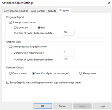
Progress
The progress of an analysis can be viewed in a report dialog opened at the start of the analysis.
Updating the progress report slows the analysis down. Therefore it is advisable to update this view more frequently during the initial runs of the model, reducing the frequency or disabling the view as the performance of the model becomes familiar.
If the option Save residuals to file is selected then the residual forces and moments at the last iteration calculated are saved in user modules in a GWA file. This GWA file can then be imported into the model using the File > Import > Text (GWA file) command to make the residuals available for tabular and contoured display.
3. Results
Output views can be accessed from View > New chart view > Nonlinear analysis > Component buckling analysis case or from Global results > Axial force / Displacement relationship.