Linear buckling analysis (modal buckling analysis)
In a modal buckling analysis, the focus is on assessing the potential for buckling in a structure under a specified load. This approach differs from modal dynamic analysis, which characterises the behavior of a structure across various conditions.
When a column undergoes increasing compressive axial load, its capacity to withstand transverse load diminishes until it reaches the Euler load, beyond which it cannot support any transverse load. The ratio of the Euler load to the actual load for a given axial load represents the load factor for that mode. If the column is supported at its midpoint then the first mode will be suppressed and higher modes with corresponding higher loads factors are possible. The eigenvalue buckling analysis extends this concept from a simple column to the whole structure, to determine global modes of buckling.
Sufficient buckling modes should be selected for the buckling analysis to ensure that all the modes of concern are identified.
1. Set up the geometry and basic modelling parameters
Create a new GSA file or open an existing model. Create members, elements, nodes, restraints, etc. as per usual keeping in mind of the following implications for buckling analysis.
Restraints
It is advised to use nodal restraints. As buckling effects are three dimensional, it is inadvisable to define global restraints on the structure, as this can potentially provide an artificial degree of stiffness to the model. To add nodal restraints, select Nodes and modify supports conditions under Properties pane > Restraints.
Releases
If you want to avoid transferring bending moments, you can add releases to the ends of elements; go to Properties pane > Releases.
Meshing members
Modal buckling analysis can only capture mode shapes where an analysis element’s end nodes move. In order to capture buckling within a single member it is advisable to mesh it in a way such that there are at least two elements per member.
To change the mesh size, select the member and go to the Properties pane to modify the analysis element size.
To generate analysis elements from the members, use the Create elements from members tool from Model > Coordination tools > Create elements from members or use the toolbar shortcut.
Checking the model with a linear static analysis
In most cases a buckling analysis follows on from a linear static analysis, so a model set up for static analysis is the normal starting point. To perform a modal buckling analysis task, it is not necessary to perform a static analysis task first, but it is recommended to do so for checking the applied load. Performing this task first also enables seeing how the structure deforms under this load and provides a better overview and control of the structural behaviour.
2. Setting up the buckling analysis task
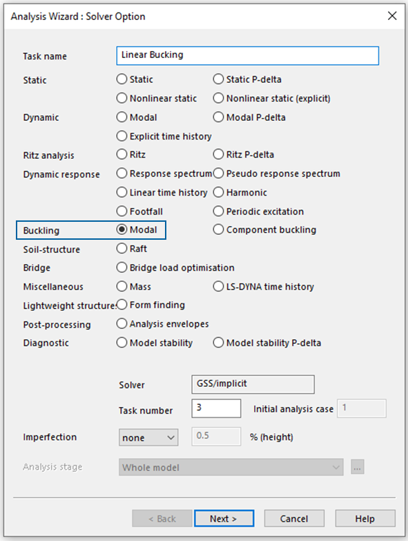
A buckling analysis is set up using the Analysis wizard. To access this, go to the Data tab of the Explorer pane and select Tasks and cases > Analysis task. Right click then select New analysis task to bring up the Analysis wizard. From here you can choose the modal buckling option.
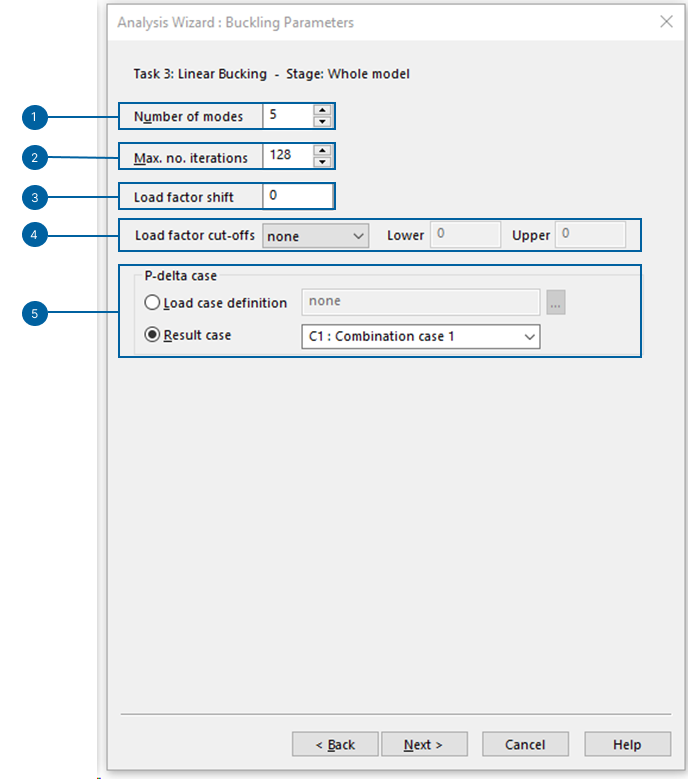
Bucking parameters
1. Define number of modes: The number of modes needed varies depending on the structure and the intended use of the modal results. In simple structures or when only the frequency of the fundamental mode is needed, a few modes will suffice. For larger and more complex structures, however, it may be necessary to analyse up to 100 modes or more.
2. Max. no. iterations: All eigensolvers are iterative. This parameter determines the maximum number of iterations permitted. In certain buckling analyses, it might be necessary to raise this value. Adjustment of the maximum number of iterations can be done through the Advanced settings dialog. While the standard value is usually sufficient, it can be increased for very complex structures.
3. Load factor shift: The load factor shift specifies the load factor around which the modes are calculated. For example, a load factor shift of 5 will find the buckling cases closest to 5, multiplied by the applied load.
4. Load factor cut-offs: The cut-offs allows for load factors outside the range of interest to be discarded. These buckling modes will still be calculated but the results are discarded rather than stored. A lower cut-off of zero will ensure that negative modes (i.e. buckling due to load reversal) are ignored. Note that these are absolute values and not relative to the load factor shift.
5. P-delta case: the buckling resistance of a structure is related to the load acting on it. The load to be used for a buckling analysis can be derived from a single load case or it can be derived from a result case.
In a P-delta analysis there is a geometric or differential stiffness in addition to the normal structure stiffness. The geometric stiffness is derived from the forces in the structure, so the solution requires two passes. The first pass calculates the internal forces, enabling the establishment of geometric stiffness for the second pass, which then resolves the modes. The GSA solver streamlines both passes within a single solution procedure.
Note: If different loads or load combinations are to be investigated, different tasks with different loads are required.
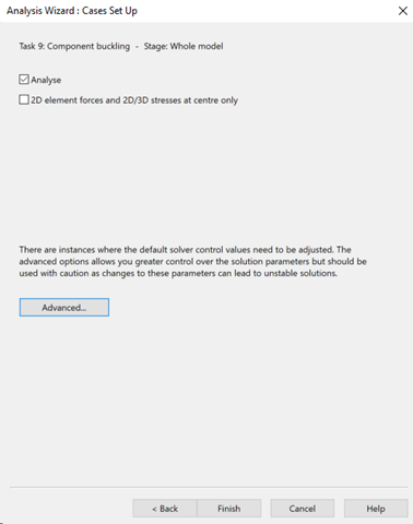
Advanced solver settings
With the advanced solver setting you can access different tabs to fine tune the analysis. In the most common cases the default values are sufficient.
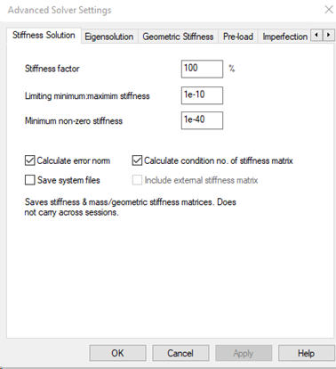
Stiffness solution
GSA uses a matrix solver for several solver options. Some options allow adjustments to be made to the assembly of the stiffness matrix.
See the References entry on Advanced solver settings for more information on this topic.
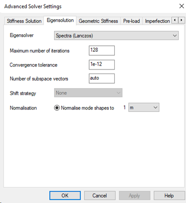
Eigensolution
Both modal dynamic analysis and buckling analysis use an eigensolver. These are iterative so it is useful to be able to control the solution procedure.
See the References entry on Eigensolution solver settings for more information on this topic.
Geometric stiffness
See the References entry on Geometric stiffness solver settings for more information on this topic.
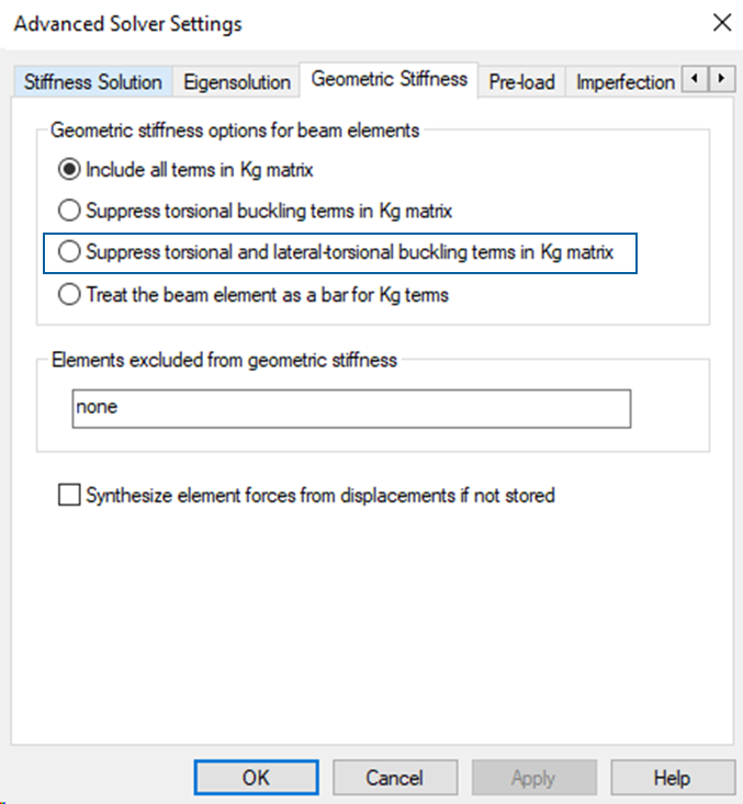
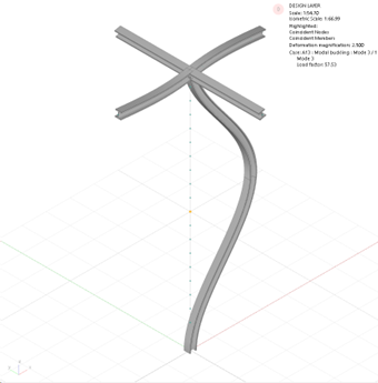
Note: If local torsional and lateral torsional buckling modes are not required for the analyses, they can be suppressed with the option Suppress torsional and lateral torsional buckling term in Kg matrix. To clarify this feature, see the following two examples: Figure 1: Include all terms in Kg matrix, Figure 2: Suppress torsional and lateral torsional buckling term in Kg matrix.
Fig. 1: Include all terms in Kg matrix
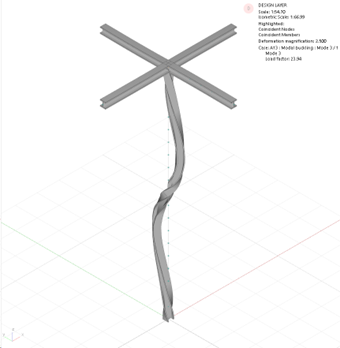
Fig.2: Suppress torsional and lateral torsional buckling term in Kg matrix
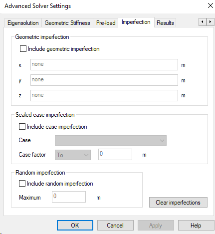
Pre-load
See the References entry on Advanced solver settings: Imperfections for more information on this topic.
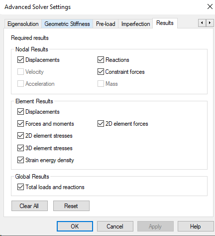
Results
GSA can calculate a large range of results. However not all of these results may be required. This allows for a selection of particular results to be stored.
See the References entry on Solver results for more information on this topic.
3. Results evaluation
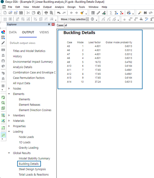
The most important result of a modal buckling analysis is the load factor (sometimes called the buckling factor). The critical buckling load (Euler´s load) is obtained by multiplying the acting loads by the load factor.
For each buckling mode a multiplication factor is defined. Go to the Output tab of the Explorer pane and select Global results > Buckling details for an overview of these values.
Alternatively, each buckling mode and the corresponding buckling load factor can also be displayed graphically, directly in the graphical interface. The advantage of this is that you can see the buckling shape and not just the buckling load factor. The bucking shape represents the last configuration of equilibrium before buckling occurs.
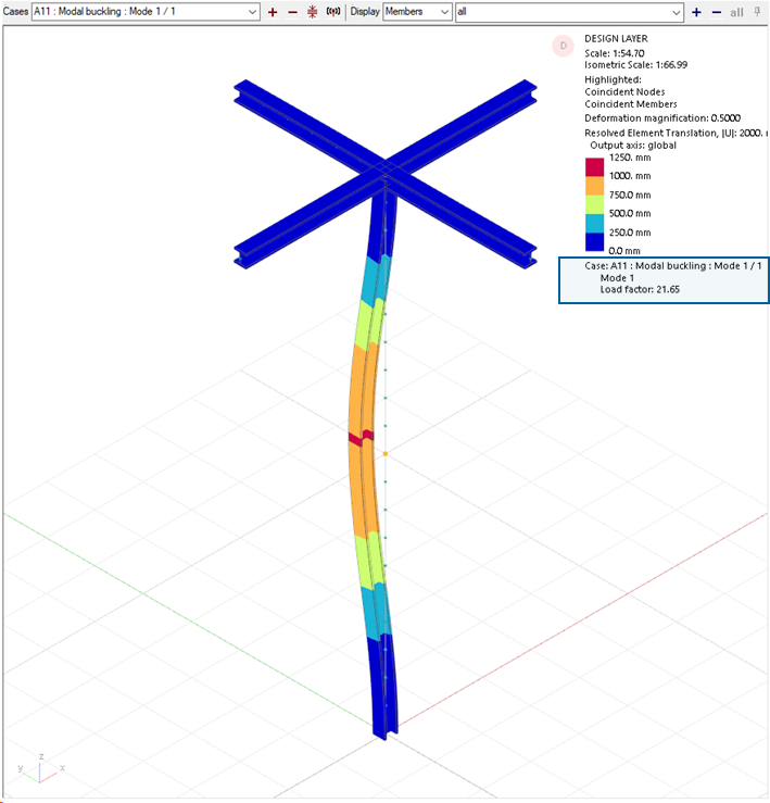
The results for buckling and static analyses are similar, but the way we interpret the results is different.
Displacements represent the mode shape, rather than an actual deflection form, and are arbitrarily scaled to give a maximum displacement of typically 1m. In addition to modal displacements, forces and reactions, there are buckling details. These are results with information such as load factor, modal stiffness and geometric stiffness.
Typically, negative eigenvalues mean that buckling cannot occur under the loading as applied. If the loading is reversed so that tension and compression are reversed in the structure, then the load factors become positive.
If the magnitude of the load factors is greater than 10 then the effects of buckling can generally be ignored. For values between 1 and 10 further checks are required.
The load factor should not be considered as a factor of safety against buckling. Instead, always acknowledge the risk of buckling and adjust accordingly, especially if the load factor is below 10.
4. Limitations
Modal buckling analysis is applicable only to linear elements. Tie and strut elements are treated as bars for buckling analysis. In the GSA solver, cable elements generally behave like tie elements. So in buckling analysis, cables are assumed to behave similarly to bar elements, making their geometric stiffness identical. This approach may result in an overestimation of the load factors.